| Title: | Intensive Care Unit Data with R |
| Description: | Focused on (but not exclusive to) data sets hosted on PhysioNet (https://physionet.org), 'ricu' provides utilities for download, setup and access of intensive care unit (ICU) data sets. In addition to functions for running arbitrary queries against available data sets, a system for defining clinical concepts and encoding their representations in tabular ICU data is presented. |
| Version: | 0.5.6 |
| License: | GPL-3 |
| Encoding: | UTF-8 |
| Language: | en-US |
| URL: | https://github.com/eth-mds/ricu, https://physionet.org |
| BugReports: | https://github.com/eth-mds/ricu/issues |
| Depends: | R (≥ 3.4.0) |
| Imports: | data.table, curl, assertthat, fst, readr, jsonlite, methods, stats, prt (≥ 0.1.2), tibble, backports, rlang, vctrs, cli (≥ 2.1.0), fansi, openssl, utils |
| Suggests: | xml2, covr, testthat (≥ 3.0.0), withr, mockthat, pkgload, mimic.demo, eicu.demo, progress, knitr, rmarkdown, ggplot2, cowplot, survival, forestmodel, rticles, kableExtra, units, pdftools, magick, pillar |
| RoxygenNote: | 7.2.3 |
| Additional_repositories: | https://eth-mds.github.io/physionet-demo |
| VignetteBuilder: | knitr |
| Config/testthat/edition: | 3 |
| NeedsCompilation: | no |
| Packaged: | 2023-09-04 13:46:08 UTC; nbennett |
| Author: | Nicolas Bennett [aut, cre], Drago Plecko [aut], Ida-Fong Ukor [aut] |
| Maintainer: | Nicolas Bennett <r@nbenn.ch> |
| Repository: | CRAN |
| Date/Publication: | 2023-09-04 18:40:03 UTC |
ricu: Intensive Care Unit Data with R
Description
Focused on (but not exclusive to) data sets hosted on PhysioNet (https://physionet.org), 'ricu' provides utilities for download, setup and access of intensive care unit (ICU) data sets. In addition to functions for running arbitrary queries against available data sets, a system for defining clinical concepts and encoding their representations in tabular ICU data is presented.
Author(s)
Maintainer: Nicolas Bennett r@nbenn.ch
Authors:
Drago Plecko drago.plecko@stat.math.ethz.ch
Ida-Fong Ukor ida-fong.ukor@monashhealth.org
See Also
Useful links:
Report bugs at https://github.com/eth-mds/ricu/issues
Internal item callback utilities
Description
The utility function add_concept() is exported for convenience when adding
external datasets and integrating concepts that require other concepts.
While this could be solves by defining a rec_concpt, in some scenarios
this might not be ideal, as it might be only required that itm
implementations for certain data sources require additional information.
Examples for this include vasopressor rates which might rely on patient
weight, and blood cell counts when expressed as ratio. For performance
reasons, the pulled in concept is internally cached, as this might be used
unchanged many times, when loading several concepts that need to pull in
the given concept. Persistence of cache is session-level and therefore this
utility is intended to be used somewhat sparingly.
Usage
add_concept(x, env, concept, var_name = concept, aggregate = NULL)

add_weight(x, env, var_name = "weight")

calc_dur(x, val_var, min_var, max_var, grp_var = NULL)

combine_callbacks(...)
Arguments
x |
Object in loading |
env |
Data source environment as available as |
concept |
String valued concept name that will be loaded from the default dictionary |
var_name |
String valued variable name |
aggregate |
Forwarded to |
val_var |
String valued column name corresponding to the value variable |
min_var, max_var |
Column names denoting start and end times |
grp_var |
Optional grouping variable (for example linking infusions) |
... |
Functions which will be successively applied |
Value
A copy of x with the requested concept merged in.
Data attach utilities
Description
Making a dataset available to ricu consists of 3 steps: downloading
(download_src()), importing (import_src()) and attaching
(attach_src()). While downloading and importing are one-time procedures,
attaching of the dataset is repeated every time the package is loaded.
Briefly, downloading loads the raw dataset from the internet (most likely
in .csv format), importing consists of some preprocessing to make the
data available more efficiently and attaching sets up the data for use by
the package.
Usage
attach_src(x, ...)

## S3 method for class 'src_cfg'
attach_src(x, assign_env = NULL, data_dir = src_data_dir(x), ...)

## S3 method for class 'character'
attach_src(x, assign_env = NULL, data_dir = src_data_dir(x), ...)

detach_src(x)

setup_src_env(x, ...)

## S3 method for class 'src_cfg'
setup_src_env(x, data_dir = src_data_dir(x), link_env = NULL, ...)
Arguments
x |
Data source to attach |
... |
Forwarded to further calls to |
assign_env, link_env |
Environment in which the data source will become available |
data_dir |
Directory used to look for |
Details
Attaching a dataset sets up two types of S3 classes: a single src_env
object, containing as many src_tbl objects as tables are associated with
the dataset. A src_env is an environment with an id_cfg attribute, as
well as sub-classes as specified by the data source class_prefix
configuration setting (see load_src_cfg()). All src_env objects created
by calling attach_src() represent environments that are direct
descendants of the data environment and are bound to the respective
dataset name within that environment. For more information on src_env and
src_tbl objects, refer to new_src_tbl().
If set up correctly, it is not necessary for the user to directly call
attach_src(). When the package is loaded, the default data sources (see
auto_attach_srcs()) are attached automatically. This default can be
controlled by setting as environment variable RICU_SRC_LOAD a comma
separated list of data source names before loading the library. Setting
this environment variable as
Sys.setenv(RICU_SRC_LOAD = "mimic_demo,eicu_demo")
will change the default of loading both MIMIC-III and eICU, alongside the
respective demo datasets, as well as HiRID and AUMC, to just the two demo
datasets. For setting an environment variable upon startup of the R
session, refer to base::.First.sys().
Attaching a dataset during package namespace loading will both instantiate
a corresponding src_env in the data environment and for convenience
also assign this object into the package namespace, such that for example
the MIMIC-III demo dataset not only is available as
ricu::data::mimic_demo, but also as ricu::mimic_demo (or if the package
namespace is attached, simply as mimic_demo). Dataset attaching using
attach_src() does not need to happen during namespace loading, but can be
triggered by the user at any time. If such a convenience link as described
above is desired by the user, an environment such as .GlobalEnv has to be
passed as assign_env to attach_src().
Data sets are set up as src_env objects irrespective of whether all (or
any) of the required data is available. If some (or all) data is missing,
the user is asked for permission to download in interactive sessions and an
error is thrown in non-interactive sessions. Downloading demo datasets
requires no further information but access to full-scale datasets (even
though they are publicly available) is guarded by access credentials (see
download_src()).
While attach_src() provides the main entry point, src_env objects are
instantiated by the S3 generic function setup_src_env() and the wrapping
function serves to catch errors that might be caused by config file parsing
issues as to not break attaching of the package namespace. Apart form this,
attach_src() also provides the convenience linking into the package
namespace (or a user-specified environment) described above.
A src_env object created by setup_src_env() does not directly contain
src_tbl objects bound to names, but rather an active binding (see
base::makeActiveBinding()) per table. These active bindings check for
availability of required files and evaluate to corresponding src_tbl
objects if these checks are passed and ask for user input otherwise. As
src_tbl objects are intended to be read-only, assignment is not possible
except for the value NULL which resets the internally cached src_tbl
that is created on first successful access.
Value
Both attach_src() and setup_src_env() are called for side
effects and therefore return invisibly. While attach_src() returns NULL,
setup_src_env() returns the newly created src_env object.
Examples
## Not run:

Sys.setenv(RICU_SRC_LOAD = "")
library(ricu)

ls(envir = data)
exists("mimic_demo")

attach_src("mimic_demo", assign_env = .GlobalEnv)

ls(envir = data)
exists("mimic_demo")

mimic_demo


## End(Not run)
ICU class data reshaping
Description
Utilities for reshaping id_tbl and ts_tbl objects.
Usage
cbind_id_tbl(
  ...,
  keep.rownames = FALSE,
  check.names = FALSE,
  key = NULL,
  stringsAsFactors = FALSE
)

rbind_id_tbl(..., use.names = TRUE, fill = FALSE, idcol = NULL)

## S3 method for class 'id_tbl'
merge(x, y, by = NULL, by.x = NULL, by.y = NULL, ...)

## S3 method for class 'id_tbl'
split(x, ...)

rbind_lst(x, ...)

merge_lst(x)

unmerge(x, col_groups = as.list(data_vars(x)), by = meta_vars(x), na_rm = TRUE)
Arguments
... |
Objects to combine |
keep.rownames, check.names, key, stringsAsFactors |
Forwarded to data.table::data.table |
use.names, fill, idcol |
Forwarded to data.table::rbindlist |
x, y |
Objects to combine |
by, by.x, by.y |
Column names used for combining data |
col_groups |
A list of character vectors defining the grouping of non-by columns |
na_rm |
Logical flag indicating whether to remove rows that have all
missing entries in the respective |
Value
Either id_tbl or ts_tbl objects (depending on inputs) or lists
thereof in case of split() and unmerge().
Switch between id types
Description
ICU datasets such as MIMIC-III or eICU typically represent patients by
multiple ID systems such as patient IDs, hospital stay IDs and ICU
admission IDs. Even if the raw data is available in only one such ID
system, given a mapping of IDs alongside start and end times, it is
possible to convert data from one ID system to another. The function
change_id() provides such a conversion utility, internally either
calling upgrade_id() when moving to an ID system with higher cardinality
and downgrade_id() when the target ID system is of lower cardinality
Usage
change_id(x, target_id, src, ..., keep_old_id = TRUE, id_type = FALSE)

upgrade_id(x, target_id, src, cols = time_vars(x), ...)

downgrade_id(x, target_id, src, cols = time_vars(x), ...)

## S3 method for class 'ts_tbl'
upgrade_id(x, target_id, src, cols = time_vars(x), ...)

## S3 method for class 'id_tbl'
upgrade_id(x, target_id, src, cols = time_vars(x), ...)

## S3 method for class 'ts_tbl'
downgrade_id(x, target_id, src, cols = time_vars(x), ...)

## S3 method for class 'id_tbl'
downgrade_id(x, target_id, src, cols = time_vars(x), ...)
Arguments
x |
|
target_id |
The destination id name |
src |
Passed to |
... |
Passed to |
keep_old_id |
Logical flag indicating whether to keep the previous ID column |
id_type |
Logical flag indicating whether |
cols |
Column names that require time-adjustment |
Details
In order to provide ID system conversion for a data source, the (internal)
function id_map() must be able to construct an ID mapping for that data
source. Constructing such a mapping can be expensive w.r.t. the frequency
it might be re-used and therefore, id_map() provides caching
infrastructure. The mapping itself is constructed by the (internal)
function id_map_helper(), which is expected to provide source and
destination ID columns as well as start and end columns corresponding to
the destination ID, relative to the source ID system. In the following
example, we request for mimic_demo, with ICU stay IDs as source and
hospital admissions as destination IDs.
id_map_helper(mimic_demo, "icustay_id", "hadm_id")
#> # An `id_tbl`: 136 x 4
#> # Id var:      `icustay_id`
#>     icustay_id hadm_id hadm_id_start hadm_id_end
#>          <int>   <int> <drtn>        <drtn>
#> 1       201006  198503  -3290 mins    9114 mins
#> 2       201204  114648     -2 mins    6949 mins
#> 3       203766  126949  -1336 mins    8818 mins
#> 4       204132  157609     -1 mins   10103 mins
#> 5       204201  177678   -368 mins    9445 mins
#> ...
#> 132     295043  170883 -10413 mins   31258 mins
#> 133     295741  176805     -1 mins    3153 mins
#> 134     296804  110244  -1294 mins    4599 mins
#> 135     297782  167612     -1 mins     207 mins
#> 136     298685  151323     -1 mins   19082 mins
#> # i 131 more rows
Both start and end columns encode the hospital admission windows relative to each corresponding ICU stay start time. It therefore comes as no surprise that most start times are negative (hospital admission typically occurs before ICU stay start time), while end times are often days in the future (as hospital discharge typically occurs several days after ICU admission).
In order to use the ID conversion infrastructure offered by ricu for a
new dataset, it typically suffices to provide an id_cfg entry in the
source configuration (see load_src_cfg()), outlining the available ID
systems alongside an ordering, as well as potentially a class specific
implementation of id_map_helper() for the given source class, specifying
the corresponding time windows in 1 minute resolution (for every possible
pair of IDs).
While both up- and downgrades for id_tbl objects, as well as downgrades
for ts_tbl objects are simple merge operations based on the ID mapping
provided by id_map(), ID upgrades for ts_tbl objects are slightly more
involved. As an example, consider the following setting: we have data
associated with hadm_id IDs and times relative to hospital admission:
               1      2       3        4       5       6        7      8
data        ---*------*-------*--------*-------*-------*--------*------*---
               3h    10h     18h      27h     35h     43h      52h    59h

                                         HADM_1
            0h     7h                26h        37h             53h      62h
hadm_id     |-------------------------------------------------------------|
icustay_id         |------------------|          |---------------|
                   0h                19h         0h             16h
                           ICU_1                       ICU_2
The mapping of data points from hadm_id to icustay_id is created as
follows: ICU stay end times mark boundaries and all data that is recorded
after the last ICU stay ended is assigned to the last ICU stay. Therefore
data points 1-3 are assigned to ICU_1, while 4-8 are assigned to ICU_2.
Times have to be shifted as well, as timestamps are expected to be relative
to the current ID system. Data points 1-3 therefore are assigned to time
stamps -4h, 3h and 11h, while data points 4-8 are assigned to -10h, -2h,
6h, 15h and 22h. Implementation-wise, the mapping is computed using an
efficient data.table rolling join.
Value
An object of the same type as x with modified IDs.
Examples
if (require(mimic.demo)) {
tbl <- mimic_demo$labevents
dat <- load_difftime(tbl, itemid == 50809, c("charttime", "valuenum"))
dat

change_id(dat, "icustay_id", tbl, keep_old_id = FALSE)
}
Internal utilities for ICU data classes
Description
Internal utilities for ICU data classes
Usage
col_renamer(x, new, old = colnames(x), skip_absent = FALSE, by_ref = FALSE)
Arguments
x |
Object to query |
new, old |
Replacement names and existing column names for renaming columns |
skip_absent |
Logical flag for ignoring non-existent column names |
by_ref |
Logical flag indicating whether to perform the operation by reference |
ICU datasets
Description
The Laboratory for Computational Physiology (LCP) at MIT hosts several large-scale databases of hospital intensive care units (ICUs), two of which can be either downloaded in full (MIMIC-III and eICU ) or as demo subsets (MIMIC-III demo and eICU demo), while a third data set is available only in full (HiRID ). While demo data sets are freely available, full download requires credentialed access which can be gained by applying for an account with PhysioNet . Even though registration is required, the described datasets are all publicly available. With AmsterdamUMCdb , a non-PhysioNet hosted data source is available as well. As with the PhysioNet datasets, access is public but has to be granted by the data collectors.
Usage
data
Format
The exported data environment contains all datasets that have been made
available to ricu. For datasets that are attached during package loading
(see attach_src()), shortcuts to the datasets are set up in the package
namespace, allowing the object ricu::data::mimic_demo to be accessed as
ricu::mimic_demo (or in case the package namespace has been attached,
simply as mimic_demo). Datasets that are made available after the package
namespace has been sealed will have their proxy object by default located
in .GlobalEnv. Datasets are represented by src_env
objects, while individual tables are src_tbl and do not
represent in-memory data, but rather data stored on disk, subsets of which
can be loaded into memory.
Details
Setting up a dataset for use with ricu requires a configuration object.
For the included datasets, configuration can be loaded from
system.file("extdata", "config", "data-sources.json", package = "ricu")
by calling load_src_cfg() and for dataset that are external to ricu,
additional configuration can be made available by setting the environment
variable RICU_CONFIG_PATH (for more information, refer to
load_src_cfg()). Using the dataset configuration object, data can be
downloaded (download_src()), imported (import_src()) and attached
(attach_src()). While downloading and importing are one-time procedures,
attaching of the dataset is repeated every time the package is loaded.
Briefly, downloading loads the raw dataset from the internet (most likely
in .csv format), importing consists of some preprocessing to make the
data available more efficiently (by converting it to .fst
format) and attaching sets up the data for use by the package. For more
information on the individual steps, refer to the respective documentation
pages.
A dataset that has been successfully made available can interactively be
explored by typing its name into the console and individual tables can be
inspected using the $ function. For example for the MIMIC-III demo
dataset and the icustays table, this gives
mimic_demo
#> <mimic_demo_env[25]>
#>         admissions            callout         caregivers        chartevents
#>         [129 x 19]          [77 x 24]        [7,567 x 4]     [758,355 x 15]
#>          cptevents              d_cpt    d_icd_diagnoses   d_icd_procedures
#>       [1,579 x 12]          [134 x 9]       [14,567 x 4]        [3,882 x 4]
#>            d_items         d_labitems     datetimeevents      diagnoses_icd
#>      [12,487 x 10]          [753 x 6]      [15,551 x 14]        [1,761 x 5]
#>           drgcodes           icustays     inputevents_cv     inputevents_mv
#>          [297 x 8]         [136 x 12]      [34,799 x 22]      [13,224 x 31]
#>          labevents microbiologyevents       outputevents           patients
#>       [76,074 x 9]       [2,003 x 16]      [11,320 x 13]          [100 x 8]
#>      prescriptions procedureevents_mv     procedures_icd           services
#>      [10,398 x 19]         [753 x 25]          [506 x 5]          [163 x 6]
#>          transfers
#>         [524 x 13]
mimic_demo$icustays
#> # <mimic_tbl>: [136 x 12]
#> # ID options:  subject_id (patient) < hadm_id (hadm) < icustay_id (icustay)
#> # Defaults:    `intime` (index), `last_careunit` (val)
#> # Time vars:   `intime`, `outtime`
#>     row_id subject_id hadm_id icustay_id dbsource   first_careunit last_careunit
#>      <int>      <int>   <int>      <int> <chr>      <chr>          <chr>
#> 1    12742      10006  142345     206504 carevue    MICU           MICU
#> 2    12747      10011  105331     232110 carevue    MICU           MICU
#> 3    12749      10013  165520     264446 carevue    MICU           MICU
#> 4    12754      10017  199207     204881 carevue    CCU            CCU
#> 5    12755      10019  177759     228977 carevue    MICU           MICU
#> ...
#> 132  42676      44083  198330     286428 metavision CCU            CCU
#> 133  42691      44154  174245     217724 metavision MICU           MICU
#> 134  42709      44212  163189     239396 metavision MICU           MICU
#> 135  42712      44222  192189     238186 metavision CCU            CCU
#> 136  42714      44228  103379     217992 metavision SICU           SICU
#> # i 131 more rows
#> # i 5 more variables: first_wardid <int>, last_wardid <int>, intime <dttm>,
#> #   outtime <dttm>, los <dbl>
Table subsets can be loaded into memory for example using the
base::subset() function, which uses non-standard evaluation (NSE) to
determine a row-subsetting. This design choice stems form the fact that
some tables can have on the order of 10^8 rows, which makes loading full
tables into memory an expensive operation. Table subsets loaded into
memory are represented as data.table objects.
Extending the above example, if only ICU stays corresponding to the patient
with subject_id == 10124 are of interest, the respective data can be
loaded as
subset(mimic_demo$icustays, subject_id == 10124)
#>    row_id subject_id hadm_id icustay_id dbsource first_careunit last_careunit
#> 1:  12863      10124  182664     261764  carevue           MICU          MICU
#> 2:  12864      10124  170883     222779  carevue           MICU          MICU
#> 3:  12865      10124  170883     295043  carevue            CCU           CCU
#> 4:  12866      10124  170883     237528  carevue           MICU          MICU
#>    first_wardid last_wardid              intime             outtime     los
#> 1:           23          23 2192-03-29 10:46:51 2192-04-01 06:36:00  2.8258
#> 2:           50          50 2192-04-16 20:58:32 2192-04-20 08:51:28  3.4951
#> 3:            7           7 2192-04-24 02:29:49 2192-04-26 23:59:45  2.8958
#> 4:           23          23 2192-04-30 14:50:44 2192-05-15 23:34:21 15.3636
Much care has been taken to make ricu extensible to new datasets. For
example the publicly available ICU database AmsterdamUMCdb
provided by the Amsterdam University Medical Center, currently is not part
of the core datasets of ricu, but code for integrating this dataset is
available on github.
MIMIC-III
The Medical Information Mart for Intensive Care (MIMIC) database holds detailed clinical data from roughly 60,000 patient stays in Beth Israel Deaconess Medical Center (BIDMC) intensive care units between 2001 and 2012. The database includes information such as demographics, vital sign measurements made at the bedside (~1 data point per hour), laboratory test results, procedures, medications, caregiver notes, imaging reports, and mortality (both in and out of hospital). For further information, please refer to the MIMIC-III documentation.
The corresponding
demo dataset
contains the full data of a randomly selected subset of 100 patients from
the patient cohort with conformed in-hospital mortality. The only notable
data omission is the noteevents table, which contains unstructured text
reports on patients.
eICU
More recently, Philips Healthcare and LCP began assembling the eICU Collaborative Research Database as a multi-center resource for ICU data. Combining data of several critical care units throughout the continental United States from the years 2014 and 2015, this database contains de-identified health data associated with over 200,000 admissions, including vital sign measurements, care plan documentation, severity of illness measures, diagnosis information, and treatment information. For further information, please refer to the eICU documentation .
For the demo subset, data associated with ICU stays for over 2,500 unit stays selected from 20 of the larger hospitals is included. An important caveat that applied to the eICU-based datasets is considerable variability among the large number of hospitals in terms of data availability.
HiRID
Moving to higher time-resolution, HiRID is a freely accessible critical care dataset containing data relating to almost 34,000 patient admissions to the Department of Intensive Care Medicine of the Bern University Hospital, Switzerland. The dataset contains de-identified demographic information and a total of 681 routinely collected physiological variables, diagnostic test results and treatment parameters, collected during the period from January 2008 to June 2016. Dependent on the type of measurement, time resolution can be on the order of 2 minutes.
AmsterdamUMCdb
With similar time-resolution (for vital-sign measurements) as HiRID, AmsterdamUMCdb contains data from 23,000 admissions of adult patients from 2003-2016 to the department of Intensive Care, of Amsterdam University Medical Center. In total, nearly 10^9^ individual observations consisting of vitals signs, clinical scoring systems, device data and lab results data, as well as nearly 5*10^6^ million medication entries, alongside de-identified demographic information corresponding to the 20,000 individual patients is spread over 7 tables.
MIMIC-IV
With the recent v1.0 release of MIMIC-IV, experimental support has been
added in ricu. Building on the success of MIMIC-III, this next iteration
contains data on patients admitted to an ICU or the emergency department
between 2008 - 2019 at BIDMC. Therefore, relative to MIMIC-III, patients
admitted prior to 2008 (whose data is stored in a CareVue-based system) has
been removed, while data onward of 2012 has been added. This simplifies
data queries considerably, as the CareVue/MetaVision data split in MIMIC-III
no longer applies. While addition of ED data is planned, this is not part
of the initial v1.0 release and currently is not supported by ricu. For
further information, please refer to the MIMIC-III documentation .
References
Johnson, A., Pollard, T., & Mark, R. (2016). MIMIC-III Clinical Database (version 1.4). PhysioNet. https://doi.org/10.13026/C2XW26.
MIMIC-III, a freely accessible critical care database. Johnson AEW, Pollard TJ, Shen L, Lehman L, Feng M, Ghassemi M, Moody B, Szolovits P, Celi LA, and Mark RG. Scientific Data (2016). DOI: 10.1038/sdata.2016.35.
Johnson, A., Pollard, T., Badawi, O., & Raffa, J. (2019). eICU Collaborative Research Database Demo (version 2.0). PhysioNet. https://doi.org/10.13026/gxmm-es70.
The eICU Collaborative Research Database, a freely available multi-center database for critical care research. Pollard TJ, Johnson AEW, Raffa JD, Celi LA, Mark RG and Badawi O. Scientific Data (2018). DOI: http://dx.doi.org/10.1038/sdata.2018.178.
Faltys, M., Zimmermann, M., Lyu, X., Hüser, M., Hyland, S., Rätsch, G., & Merz, T. (2020). HiRID, a high time-resolution ICU dataset (version 1.0). PhysioNet. https://doi.org/10.13026/hz5m-md48.
Hyland, S.L., Faltys, M., Hüser, M. et al. Early prediction of circulatory failure in the intensive care unit using machine learning. Nat Med 26, 364–373 (2020). https://doi.org/10.1038/s41591-020-0789-4
Thoral PJ, Peppink JM, Driessen RH, et al (2020) AmsterdamUMCdb: The First Freely Accessible European Intensive Care Database from the ESICM Data Sharing Initiative. https://www.amsterdammedicaldatascience.nl.
Elbers, Dr. P.W.G. (Amsterdam UMC) (2019): AmsterdamUMCdb v1.0.2. DANS. https://doi.org/10.17026/dans-22u-f8vd
Johnson, A., Bulgarelli, L., Pollard, T., Horng, S., Celi, L. A., & Mark, R. (2021). MIMIC-IV (version 1.0). PhysioNet. https://doi.org/10.13026/s6n6-xd98.
Goldberger, A., Amaral, L., Glass, L., Hausdorff, J., Ivanov, P. C., Mark, R., ... & Stanley, H. E. (2000). PhysioBank, PhysioToolkit, and PhysioNet: Components of a new research resource for complex physiologic signals. Circulation (Online). 101 (23), pp. e215–e220.
File system utilities
Description
Determine the location where to place data meant to persist between individual sessions.
Usage
data_dir(subdir = NULL, create = TRUE)

src_data_dir(srcs)

auto_attach_srcs()

config_paths()

get_config(name, cfg_dirs = config_paths(), combine_fun = c, ...)

set_config(x, name, dir = file.path("inst", "extdata", "config"), ...)
Arguments
subdir |
A string specifying a directory that will be made sure to exist below the data directory. |
create |
Logical flag indicating whether to create the specified directory |
srcs |
Character vector of data source names, an object for which an
|
name |
File name of the configuration file ( |
cfg_dirs |
Character vector of directories searched for config files |
combine_fun |
If multiple files are found, a function for combining returned lists |
... |
Passed to |
x |
Object to be written |
dir |
Directory to write the file to (created if non-existent) |
Details
For data, the default location depends on the operating system as
| Platform | Location |
| Linux | ~/.local/share/ricu |
| macOS | ~/Library/Application Support/ricu |
| Windows | %LOCALAPPDATA%/ricu |
If the default storage directory does not exists, it will only be created upon user consent (requiring an interactive session).
The environment variable RICU_DATA_PATH can be used to overwrite the
default location. If desired, this variable can be set in an R startup file
to make it apply to all R sessions. For example, it could be set within:
A project-local
.Renviron;The user-level
.Renviron;A file at
$(R RHOME)/etc/Renviron.site.
Any directory specified as environment variable will recursively be created.
Data source directories typically are sub-directories to data_dir() named
the same as the respective dataset. For demo datasets corresponding to
mimic and eicu, file location however deviates from this scheme. The
function src_data_dir() is used to determine the expected data location
of a given dataset.
Configuration files used both for data source configuration, as well as for
dictionary definitions potentially involve multiple files that are read and
merged. For that reason, get_config() will iterate over directories
passed as cfg_dirs and look for the specified file (with suffix .json
appended and might be missing in some of the queried directories). All
found files are read by jsonlite::read_json() and the resulting lists are
combined by reduction with the binary function passed as combine_fun.
With default arguments, get_config() will simply concatenate lists
corresponding to files found in the default config locations as returned by
config_paths(): first the directory specified by the environment variable
RICU_CONFIG_PATH (if set), followed by the directory at
system.file("extdata", "config", package = "ricu")
Further arguments are passed to jsonlite::read_json(), which is called
with slightly modified defaults: simplifyVector = TRUE,
simplifyDataFrame = FALSE and simplifyMatrix = FALSE.
The utility function set_config() writes the list passed as x to file
dir/name.json, using jsonlite::write_json() also with slightly modified
defaults (which can be overridden by passing arguments as ...): null = "null", auto_unbox = TRUE and pretty = TRUE.
Whenever the package namespace is attached, a summary of dataset
availability is printed using the utility functions auto_attach_srcs()
and src_data_avail(). While the former simply returns a character vector
of data sources that are configures for automatically being set up on
package loading, the latter returns a summary of the number of available
tables per dataset.m Finally, is_data_avail() returns a named logical
vector indicating which data sources have all required data available.
Value
Functions data_dir(), src_data_dir() and config_paths() return
file paths as character vectors, auto_attach_srcs() returns a character
vector of data source names, src_data_avail() returns a data.frame
describing availability of data sources and is_data_avail() a named
logical vector. Configuration utilities get_config() and set_config()
read and write list objects to/from JSON format.
Examples
Sys.setenv(RICU_DATA_PATH = tempdir())
identical(data_dir(), tempdir())

dir.exists(file.path(tempdir(), "some_subdir"))
some_subdir <- data_dir("some_subdir")
dir.exists(some_subdir)

cfg <- get_config("concept-dict")

identical(
  cfg,
  get_config("concept-dict",
             system.file("extdata", "config", package = "ricu"))
)
Data download utilities
Description
Making a dataset available to ricu consists of 3 steps: downloading
(download_src()), importing (import_src()) and attaching
(attach_src()). While downloading and importing are one-time procedures,
attaching of the dataset is repeated every time the package is loaded.
Briefly, downloading loads the raw dataset from the internet (most likely
in .csv format), importing consists of some preprocessing to make the
data available more efficiently (by converting it to .fst
format) and attaching sets up the data for use by the package.
Usage
download_src(x, data_dir = src_data_dir(x), ...)

## S3 method for class 'src_cfg'
download_src(x, data_dir = src_data_dir(x), tables = NULL, force = FALSE, ...)

## S3 method for class 'aumc_cfg'
download_src(
  x,
  data_dir = src_data_dir(x),
  tables = NULL,
  force = FALSE,
  token = NULL,
  verbose = TRUE,
  ...
)

## S3 method for class 'character'
download_src(
  x,
  data_dir = src_data_dir(x),
  tables = NULL,
  force = FALSE,
  user = NULL,
  pass = NULL,
  verbose = TRUE,
  ...
)
Arguments
x |
Object specifying the source configuration |
data_dir |
Destination directory where the downloaded data is written to. |
... |
Generic consistency |
tables |
Character vector specifying the tables to download. If
|
force |
Logical flag; if |
token |
Download token for AmsterdamUMCdb (see 'Details') |
verbose |
Logical flag indicating whether to print progress information |
user, pass |
PhysioNet credentials; if |
Details
Downloads by ricu are focused data hosted by
PhysioNet and tools are currently available for
downloading the datasets
MIMIC-III,
eICU and
HiRID (see data). While
credentials are required for downloading any of the three datasets, demo
dataset for both MIMIC-III and eICU are available without having to log in.
Even though access to full dataset is credentialed, the datasets are in
fact publicly available. For setting up an account, please refer to the registration form.
PhysioNet credentials can either be entered in an interactive session,
passed as function arguments user/pass or as environment
variables RICU_PHYSIONET_USER/RICU_PHYSIONET_PASS. For setting
environment variables on session startup, refer to base::.First.sys() and
for setting environment variables in general, refer to base::Sys.setenv()
If the openssl package is available, SHA256 hashes of downloaded files are
verified using openssl::sha256().
Demo datasets MIMIC-III demo and eICU demo can either be installed as R packages directly by running
install.packages(
  c("mimic.demo", "eicu.demo"),
  repos = "https://eth-mds.github.io/physionet-demo"
)
or downloaded and imported using download_src() and import_src().
Furthermore, ricu specifies mimic.demo and eicu.demo as Suggests
dependencies therefore, passing dependencies = TURE when calling
install.packages() for installing ricu, this will automatically install
the demo datasets as well.
While the included data downloaders are intended for data hosted by
PhysioNet, download_src() is an S3 generic function that can be extended
to new classes. Method dispatch is intended to occur on objects that
inherit from or can be coerced to src_cfg. For more information on data
source configuration, refer to load_src_cfg().
As such, with the addition of the AmsterdamUMCdb dataset, which
unfortunately is not hosted on PhysioNet, A separate downloader for that
dataset is available as well. Currently this requires both availability of
the CRAN package xml2, as well as the command line utility 7zip.
Furthermore, data access has to be requested and for
non-interactive download the download token has to be made available as
environment variable RICU_AUMC_TOKEN or passed as token argument to
download_src(). The download token can be retrieved from the URL provided
when granted access as by extracting the string followed by token=:
https://example.org/?s=download&token=0c27af59-72d1-0349-aa59-00000a8076d9
would translate to
Sys.setenv(RICU_AUMC_TOKEN = "0c27af59-72d1-0349-aa59-00000a8076d9")
If the dependencies outlined above are not fulfilled, download and archive
extraction can be carried out manually into the corresponding folder and
import_src() can be run.
Value
Called for side effects and returns NULL invisibly.
Examples
## Not run:

dir <- tempdir()
list.files(dir)

download_datasource("mimic_demo", data_dir = dir)
list.files(dir)

unlink(dir, recursive = TRUE)


## End(Not run)
Time series utility functions
Description
ICU data as handled by ricu is mostly comprised of time series data and as
such, several utility functions are available for working with time series
data in addition to a class dedicated to representing time series data (see
ts_tbl()). Some terminology to begin with: a time series is considered
to have gaps if, per (combination of) ID variable value(s), some time steps
are missing. Expanding and collapsing mean to change between
representations where time steps are explicit or encoded as interval with
start and end times. For sliding window-type operations, slide() means to
iterate over time-windows, slide_index() means to iterate over certain
time-windows, selected relative to the index and hop() means to iterate
over time-windows selected in absolute terms.
Usage
expand(
  x,
  start_var = index_var(x),
  end_var = NULL,
  step_size = time_step(x),
  new_index = start_var,
  keep_vars = NULL,
  aggregate = FALSE
)

collapse(
  x,
  id_vars = NULL,
  index_var = NULL,
  start_var = "start",
  end_var = "end",
  env = NULL,
  as_win_tbl = TRUE,
  ...
)

has_no_gaps(x)

has_gaps(...)

is_regular(x)

fill_gaps(x, limits = collapse(x), start_var = "start", end_var = "end")

remove_gaps(x)

slide(x, expr, before, after = hours(0L), ...)

slide_index(x, expr, index, before, after = hours(0L), ...)

hop(
  x,
  expr,
  windows,
  full_window = FALSE,
  lwr_col = "min_time",
  upr_col = "max_time",
  left_closed = TRUE,
  right_closed = TRUE,
  eval_env = NULL,
  ...
)
Arguments
x |
|
start_var, end_var |
Name of the columns that represent lower and upper windows bounds |
step_size |
Controls the step size used to interpolate between
|
new_index |
Name of the new index column |
keep_vars |
Names of the columns to hold onto |
aggregate |
Function for aggregating values in overlapping intervals |
id_vars, index_var |
ID and index variables |
env |
Environment used as parent to the environment used to evaluate
expressions passes as |
as_win_tbl |
Logical flag indicating whether to return a |
... |
Passed to |
limits |
A table with columns for lower and upper window bounds or a length 2 difftime vector |
expr |
Expression (quoted for |
before, after |
Time span to look back/forward |
index |
A vector of times around which windows are spanned (relative to the index) |
windows |
An |
full_window |
Logical flag controlling how the situation is handled where the sliding window extends beyond available data |
lwr_col, upr_col |
Names of columns (in |
left_closed, right_closed |
Logical flag indicating whether intervals are closed (default) or open. |
eval_env |
Environment in which |
Details
A gap in a ts_tbl object is a missing time step, i.e. a missing entry in
the sequence seq(min(index), max(index), by = interval) in at least one
group (as defined by id_vars(), where the extrema are calculated per
group. In this case, has_gaps() will return TRUE. The function
is_regular() checks whether the time series has no gaps, in addition to
the object being sorted and unique (see is_sorted() and is_unique()).
In order to transform a time series containing gaps into a regular time
series, fill_gaps() will fill missing time steps with NA values in all
data_vars() columns, while remove_gaps() provides the inverse operation
of removing time steps that consist of NA values in data_vars() columns.
An expand() operation performed on an object inheriting from data.table
yields a ts_tbl where time-steps encoded by columns start_var and
end_var are made explicit with values in keep_vars being appropriately
repeated. The inverse operation is available as collapse(), which groups
by id_vars, represents index_var as group-wise extrema in two new
columns start_var and end_var and allows for further data summary using
.... An aspect to keep in mind when applying expand() to a win_tbl
object is that values simply are repeated for all time-steps that fall into
a given validity interval. This gives correct results when a win_tbl for
example contains data on infusions as rates, but might not lead to correct
results when infusions are represented as drug amounts administered over a
given time-span. In such a scenario it might be desirable to evenly
distribute the total amount over the corresponding time steps (currently not
implemented).
Sliding-window type operations are available as slide(), slide_index()
and hop() (function naming is inspired by the CRAN package slider). The
most flexible of the three, hop takes as input a ts_tbl object x
containing the data, an id_tbl object windows, containing for each ID
the desired windows represented by two columns lwr_col and upr_col, as
well as an expression expr to be evaluated per window. At the other end
of the spectrum, slide() spans windows for every ID and available
time-step using the arguments before and after, while slide_index()
can be seen as a compromise between the two, where windows are spanned for
certain time-points, specified by index.
Value
Most functions return ts_tbl objects with the exception of
has_gaps()/has_no_gaps()/is_regular(), which return logical flags.
Examples
if (FALSE) {
tbl <- ts_tbl(x = 1:5, y = hours(1:5), z = hours(2:6), val = rnorm(5),
              index_var = "y")
exp <- expand(tbl, "y", "z", step_size = 1L, new_index = "y",
              keep_vars = c("x", "val"))
col <- collapse(exp, start_var = "y", end_var = "z", val = unique(val))
all.equal(tbl, col, check.attributes = FALSE)

tbl <- ts_tbl(x = rep(1:5, 1:5), y = hours(sequence(1:5)), z = 1:15)

win <- id_tbl(x = c(3, 4), a = hours(c(2, 1)), b = hours(c(3, 4)))
hop(tbl, list(z = sum(z)), win, lwr_col = "a", upr_col = "b")
slide_index(tbl, list(z = sum(z)), hours(c(4, 5)), before = hours(2))
slide(tbl, list(z = sum(z)), before = hours(2))

tbl <- ts_tbl(x = rep(3:4, 3:4), y = hours(sequence(3:4)), z = 1:7)
has_no_gaps(tbl)
is_regular(tbl)

tbl[1, 2] <- hours(2)
has_no_gaps(tbl)
is_regular(tbl)

tbl[6, 2] <- hours(2)
has_no_gaps(tbl)
is_regular(tbl)
}
Data loading utilities
Description
Two important tools for smoothing out differences among used datasets are
id_origin() which returns origin times for a given ID and id_map()
which returns a mapping between two ID systems alongside start and end
columns of the target ID system relative to the source ID system. As both
these function are called frequently during data loading and might involve
somewhat expensive operations, both rely on internal helper functions
(id_orig_helper() and id_map_helper()) which perform the heavy lifting
and wrap those helper functions, providing a memoization layer. When adding
a new data source, a class specific implementation of the S3 generic
function id_map_helper() might be required, as this is used during data
loading using load_id() and load_ts() via change_id().
Usage
id_origin(x, id, origin_name = NULL, copy = TRUE)

id_orig_helper(x, id)

## S3 method for class 'src_env'
id_orig_helper(x, id)

## S3 method for class 'miiv_env'
id_orig_helper(x, id)

id_windows(x, copy = TRUE)

id_win_helper(x)

## S3 method for class 'mimic_env'
id_win_helper(x)

## S3 method for class 'eicu_env'
id_win_helper(x)

## S3 method for class 'hirid_env'
id_win_helper(x)

## S3 method for class 'aumc_env'
id_win_helper(x)

## S3 method for class 'miiv_env'
id_win_helper(x)

id_map(x, id_var, win_var, in_time = NULL, out_time = NULL)

id_map_helper(x, id_var, win_var)

## S3 method for class 'src_env'
id_map_helper(x, id_var, win_var)
Arguments
x |
Object identify the ID system (passed to |
id |
ID name for which to return origin times |
origin_name |
String-valued name which will be used to label the origin column |
copy |
Logical flag indicating whether to return a copy of the memoized
|
id_var |
Type of ID all returned times are relative to |
win_var |
Type of ID for which the in/out times is returned |
in_time, out_time |
column names of the returned in/out times |
Details
For the internal datasets, id_map_helper() relies on yet another S3
generic function id_windows(), which provides a table containing all
available ID systems, as well as all ID windows for a given data source. As
for the other two functions, the same helper-function approach is in place,
with the data loading function id_win_helper(). The function
id_map_helper() is then implemented in a data source agnostic manner
(dispatching on the src_env class), providing subsetting of this larger
ID map table and ensuring timestamps are relative to the correct ID system.
For adding a new data source however, this layer can be forgone. Similarly
for id_origin(), this is used for the internal datasets in
load_difftime(). An implementation of load_difftime(), specific to a
new data source can be provided that does not rely on id_windows(),
making this function irrelevant for this specific dataset.
Value
-
id_origin()/id_orig_helper(): anid_tblwith admission time stamps corresponding to the selected ID -
id_windows()/id_win_helper(): anid_tblholding all IDs and their respective start and end times -
id_map()/id_map_helper(): anid_tblcontaining the selected IDs and depending on values passed asin_timeandout_time, start and end times of the ID passed aswin_var
Tabular ICU data classes
Description
In order to simplify handling or tabular ICU data, ricu provides
S3 classes, id_tbl, ts_tbl, and win_tbl. These classes essentially
consist of a data.table object, alongside some meta data and S3 dispatch
is used to enable more natural behavior for some data manipulation tasks.
For example, when merging two tables, a default for the by argument can
be chosen more sensibly if columns representing patient ID and timestamp
information can be identified.
Usage
id_tbl(..., id_vars = 1L)

is_id_tbl(x)

as_id_tbl(x, id_vars = NULL, by_ref = FALSE)

ts_tbl(..., id_vars = 1L, index_var = NULL, interval = NULL)

is_ts_tbl(x)

as_ts_tbl(x, id_vars = NULL, index_var = NULL, interval = NULL, by_ref = FALSE)

win_tbl(..., id_vars = NULL, index_var = NULL, interval = NULL, dur_var = NULL)

is_win_tbl(x)

as_win_tbl(
  x,
  id_vars = NULL,
  index_var = NULL,
  interval = NULL,
  dur_var = NULL,
  by_ref = FALSE
)

## S3 method for class 'id_tbl'
as.data.table(x, keep.rownames = FALSE, by_ref = FALSE, ...)

## S3 method for class 'id_tbl'
as.data.frame(x, row.names = NULL, optional = FALSE, ...)

validate_tbl(x)
Arguments
... |
forwarded to |
id_vars |
Column name(s) to be used as |
x |
Object to query/operate on |
by_ref |
Logical flag indicating whether to perform the operation by reference |
index_var |
Column name of the index column |
interval |
Time series interval length specified as scalar-valued
|
dur_var |
Column name of the duration column |
keep.rownames |
Default is |
row.names |
|
optional |
logical. If |
Details
The introduced classes are designed for several often encountered data scenarios:
-
id_tblobjects can be used to represent static (with respect to relevant time scales) patient data such as patient age and such an object is simply adata.tablecombined with a non-zero length character vector valued attribute marking the columns tracking patient ID information (id_vars). All further columns are considered as data_vars. -
ts_tblobjects are used for grouped time series data. Adata.tableobject again is augmented by attributes, including a non-zero length character vector identifying patient ID columns (id_vars), a string, tracking the column holding time-stamps (index_var) and a scalardifftimeobject determining the time-series step size interval. Again, all further columns are treated as data_vars. -
win_tbl: In addition to representing grouped time-series data as does ats_tbl,win_tblobjects also encode a validity interval for each time-stamped measurement (as dur_var). This can for example be useful when a drug is administered at a certain infusion rate for a given time period.
Owing to the nested structure of required meta data, ts_tbl inherits from
id_tbl and win_tbl from ts_tbl. Furthermore, both classes inherit from
data.table. As such, data.table reference semantics
are available for some operations, indicated by presence of a by_ref
argument. At default, value, by_ref is set to FALSE as this is in line
with base R behavior at the cost of potentially incurring unnecessary data
copies. Some care has to be taken when passing by_ref = TRUE and enabling
by reference operations as this can have side effects (see examples).
For instantiating ts_tbl objects, both index_var and interval can be
automatically determined if not specified. For the index column, the only
requirement is that a single difftime column is
present, while for the time step, the minimal difference between two
consecutive observations is chosen (and all differences are therefore
required to be multiples of the minimum difference). Similarly, for a
win_tbl, exactly two difftime columns are required
where the first is assumed to be corresponding to the index_var and the
second to the dur_var.
Upon instantiation, the data might be rearranged: columns are reordered
such that ID columns are moved to the front, followed by the index column
and a data.table::key() is set on meta columns, causing rows to be sorted
accordingly. Moving meta columns to the front is done for reasons of
convenience for printing, while setting a key on meta columns is done to
improve efficiency of subsequent transformations such as merging or grouped
operations. Furthermore, NA values in either ID or index columns are not
allowed and therefore corresponding rows are silently removed.
Coercion between id_tbl and ts_tbl (and win_tbl) by default keeps
intersecting attributes fixed and new attributes are by default inferred as
for class instantiation. Each class comes with a class-specific
implementation of the S3 generic function validate_tbl() which returns
TRUE if the object is considered valid or a string outlining the type of
validation failure that was encountered. Validity requires
inheriting from
data.tableand unique column namesfor
id_tblthat all columns specified by the non-zero length character vector holding onto theid_varsspecification are availablefor
ts_tblthat the string-valuedindex_varcolumn is available and does not intersect withid_varsand that the index column obeys the specified interval.for
win_tblthat the string-valueddur_varcorresponds to adifftimevector and is not among the columns marked as index or ID variables
Finally, inheritance can be checked by calling is_id_tbl() and
is_ts_tbl(). Note that due to ts_tbl inheriting from id_tbl,
is_id_tbl() returns TRUE for both id_tbl and ts_tbl objects (and
similarly for win_tbl), while is_ts_tbl() only returns TRUE for
ts_tbl objects.
Value
Constructors id_tbl()/ts_tbl()/win_tbl(), as well as coercion
functions as_id_tbl()/as_ts_tbl()/as_win_tbl() return
id_tbl/ts_tbl/win_tbl objects respectively,
while inheritance testers is_id_tbl()/is_ts_tbl()/is_win_tbl() return
logical flags and validate_tbl() returns either TRUE or a string
describing the validation failure.
Relationship to data.table
Both id_tbl and ts_tbl inherit from data.table and as such, functions
intended for use with data.table objects can be applied to id_tbl and
ts_tbl as well. But there are some caveats: Many functions introduced by
data.table are not S3 generic and therefore they would have to be masked
in order to retain control over how they operate on objects inheriting form
data.table. Take for example the function data.table::setnames(), which
changes column names by reference. Using this function, the name of an
index column of an id_tbl object can me changed without updating the
attribute marking the column as such and thusly leaving the object in an
inconsistent state. Instead of masking the function setnames(), an
alternative is provided as rename_cols(). In places where it is possible
to seamlessly insert the appropriate function (such as
base::names<-() or base::colnames<-()) and the responsibility for not
using data.table::setnames() in a way that breaks the id_tbl object is
left to the user.
Owing to data.table heritage, one of the functions that is often called
on id_tbl and ts_tbl objects is base S3 generic [base::[()]. As this
function is capable of modifying the object in a way that makes it
incompatible with attached meta data, an attempt is made at preserving as
much as possible and if all fails, a data.table object is returned
instead of an object inheriting form id_tbl. If for example the index
column is removed (or modified in a way that makes it incompatible with the
interval specification) from a ts_tbl, an id_tbl is returned. If
however the ID column is removed the only sensible thing to return is a
data.table (see examples).
Examples
tbl <- id_tbl(a = 1:10, b = rnorm(10))
is_id_tbl(tbl)
is_ts_tbl(tbl)

dat <- data.frame(a = 1:10, b = hours(1:10), c = rnorm(10))
tbl <- as_ts_tbl(dat, "a")
is_id_tbl(tbl)
is_ts_tbl(tbl)

tmp <- as_id_tbl(tbl)
is_ts_tbl(tbl)
is_ts_tbl(tmp)

tmp <- as_id_tbl(tbl, by_ref = TRUE)
is_ts_tbl(tbl)
is_ts_tbl(tmp)

tbl <- id_tbl(a = 1:10, b = rnorm(10))
names(tbl) <- c("c", "b")
tbl

tbl <- id_tbl(a = 1:10, b = rnorm(10))
validate_tbl(data.table::setnames(tbl, c("c", "b")))

tbl <- id_tbl(a = 1:10, b = rnorm(10))
validate_tbl(rename_cols(tbl, c("c", "b")))

tbl <- ts_tbl(a = rep(1:2, each = 5), b = hours(rep(1:5, 2)), c = rnorm(10))
tbl[, c("a", "c"), with = FALSE]
tbl[, c("b", "c"), with = FALSE]
tbl[, list(a, b = as.double(b), c)]
ICU class meta data utilities
Description
The two data classes id_tbl and ts_tbl, used by ricu to represent ICU
patient data, consist of a data.table alongside some meta data. This
includes marking columns that have special meaning and for data
representing measurements ordered in time, the step size. The following
utility functions can be used to extract columns and column names with
special meaning, as well as query a ts_tbl object regarding its time
series related meta data.
Usage
id_vars(x)

id_var(x)

id_col(x)

index_var(x)

index_col(x)

dur_var(x)

dur_col(x)

dur_unit(x)

meta_vars(x)

data_vars(x)

data_var(x)

data_col(x)

interval(x)

time_unit(x)

time_step(x)

time_vars(x)
Arguments
x |
Object to query |
Details
The following functions can be used to query an object for columns or column names that represent a distinct aspect of the data:
-
id_vars(): ID variables are one or more column names with the interaction of corresponding columns identifying a grouping of the data. Most commonly this is some sort of patient identifier. -
id_var(): This function either fails or returns a string and can therefore be used in case only a single column provides grouping information. -
id_col(): Again, in case only a single column provides grouping information, this column can be extracted using this function. -
index_var(): Suitable for use as index variable is a column that encodes a temporal ordering of observations asdifftimevector. Only a single column can be marked as index variable and this function queries ats_tblobject for its name. -
index_col(): similarly toid_col(), this function extracts the column with the given designation. As ats_tblobject is required to have exactly one column marked as index, this function always returns forts_tblobjects (and fails forid_tblobjects). -
dur_var(): Forwin_tblobjects, this returns the name of the column encoding the data validity interval. -
dur_col(): Similarly toindex_col(), this returns thedifftimevector corresponding to thedur_var(). -
meta_vars(): Forts_tblobjects, meta variables represent the union of ID and index variables (forwin_tbl, this also includes thedur_var()), while forid_tblobjects meta variables consist pf ID variables. -
data_vars(): Data variables on the other hand are all columns that are not meta variables. -
data_var(): Similarly toid_var(), this function either returns the name of a single data variable or fails. -
data_col(): Building ondata_var(), in situations where only a single data variable is present, it is returned or if multiple data column exists, an error is thrown. -
time_vars(): Time variables are all columns in an object inheriting fromdata.framethat are of typedifftime. Therefore in ats_tblobject the index column is one of (potentially) several time variables. For awin_tbl, however thedur_var()is not among thetime_vars(). -
interval(): The time series interval length is represented a scalar valueddifftimeobject. -
time_unit(): The time unit of the time series interval, represented by a string such as "hours" or "mins" (seedifftime). -
time_step(): The time series step size represented by a numeric value in the unit as returned bytime_unit().
Value
Mostly column names as character vectors, in case of id_var(),
index_var(), data_var() and time_unit() of length 1, else of variable
length. Functions id_col(), index_col() and data_col() return table
columns as vectors, while interval() returns a scalar valued difftime
object and time_step() a number.
Examples
tbl <- id_tbl(a = rep(1:2, each = 5), b = rep(1:5, 2), c = rnorm(10),
              id_vars = c("a", "b"))

id_vars(tbl)
tryCatch(id_col(tbl), error = function(...) "no luck")
data_vars(tbl)
data_col(tbl)

tmp <- as_id_tbl(tbl, id_vars = "a")
id_vars(tmp)
id_col(tmp)

tbl <- ts_tbl(a = rep(1:2, each = 5), b = hours(rep(1:5, 2)), c = rnorm(10))
index_var(tbl)
index_col(tbl)

identical(index_var(tbl), time_vars(tbl))

interval(tbl)
time_unit(tbl)
time_step(tbl)
Data import utilities
Description
Making a dataset available to ricu consists of 3 steps: downloading
(download_src()), importing (import_src()) and attaching
(attach_src()). While downloading and importing are one-time procedures,
attaching of the dataset is repeated every time the package is loaded.
Briefly, downloading loads the raw dataset from the internet (most likely
in .csv format), importing consists of some preprocessing to make the
data available more efficiently and attaching sets up the data for use by
the package.
Usage
import_src(x, ...)

## S3 method for class 'src_cfg'
import_src(
  x,
  data_dir = src_data_dir(x),
  tables = NULL,
  force = FALSE,
  verbose = TRUE,
  ...
)

## S3 method for class 'aumc_cfg'
import_src(x, ...)

## S3 method for class 'character'
import_src(
  x,
  data_dir = src_data_dir(x),
  tables = NULL,
  force = FALSE,
  verbose = TRUE,
  cleanup = FALSE,
  ...
)

import_tbl(x, ...)

## S3 method for class 'tbl_cfg'
import_tbl(
  x,
  data_dir = src_data_dir(x),
  progress = NULL,
  cleanup = FALSE,
  ...
)
Arguments
x |
Object specifying the source configuration |
... |
Passed to downstream methods (finally to readr::read_csv/readr::read_csv_chunked)/generic consistency |
data_dir |
Destination directory where the downloaded data is written to. |
tables |
Character vector specifying the tables to download. If
|
force |
Logical flag; if |
verbose |
Logical flag indicating whether to print progress information |
cleanup |
Logical flag indicating whether to remove raw csv files after conversion to fst |
progress |
Either |
Details
In order to speed up data access operations, ricu does not directly use
the PhysioNet provided CSV files, but converts all data to fst::fst()
format, which allows for random row and column access. Large tables are
split into chunks in order to keep memory requirements reasonably low.
The one-time step per dataset of data import is fairly resource intensive: depending on CPU and available storage system, it will take on the order of an hour to run to completion and depending on the dataset, somewhere between 50 GB and 75 GB of temporary disk space are required as tables are uncompressed, in case of partitioned data, rows are reordered and the data again is saved to a storage efficient format.
The S3 generic function import_src() performs import of an entire data
source, internally calling the S3 generic function import_tbl() in order
to perform import of individual tables. Method dispatch is intended to
occur on objects inheriting from src_cfg and tbl_cfg respectively. Such
objects can be generated from JSON based configuration files which contain
information such as table names, column types or row numbers, in order to
provide safety in parsing of .csv files. For more information on data
source configuration, refer to load_src_cfg().
Current import capabilities include re-saving a .csv file to .fst at
once (used for smaller sized tables), reading a large .csv file using the
readr::read_csv_chunked() API, while partitioning chunks and reassembling
sub-partitions (used for splitting a large file into partitions), as well
as re-partitioning an already partitioned table according to a new
partitioning scheme. Care has been taken to keep the maximal memory
requirements for this reasonably low, such that data import is feasible on
laptop class hardware.
Value
Called for side effects and returns NULL invisibly.
Examples
## Not run:

dir <- tempdir()
list.files(dir)

download_src("mimic_demo", dir)
list.files(dir)

import_src("mimic_demo", dir)
list.files(dir)

unlink(dir, recursive = TRUE)


## End(Not run)
Load concept data
Description
Concept objects are used in ricu as a way to specify how a clinical
concept, such as heart rate can be loaded from a data source. Building on
this abstraction, load_concepts() powers concise loading of data with
data source specific preprocessing hidden away from the user, thereby
providing a data source agnostic interface to data loading. At default
value of the argument merge_data, a tabular data structure (either a
ts_tbl or an id_tbl, depending on what kind of
concepts are requested), inheriting from
data.table, is returned, representing the data
in wide format (i.e. returning concepts as columns).
Usage
load_concepts(x, ...)

## S3 method for class 'character'
load_concepts(
  x,
  src = NULL,
  concepts = NULL,
  ...,
  dict_name = "concept-dict",
  dict_dirs = NULL
)

## S3 method for class 'integer'
load_concepts(
  x,
  src = NULL,
  concepts = NULL,
  ...,
  dict_name = "concept-dict",
  dict_dirs = NULL
)

## S3 method for class 'numeric'
load_concepts(x, ...)

## S3 method for class 'concept'
load_concepts(
  x,
  src = NULL,
  aggregate = NULL,
  merge_data = TRUE,
  verbose = TRUE,
  ...
)

## S3 method for class 'cncpt'
load_concepts(x, aggregate = NULL, ..., progress = NULL)

## S3 method for class 'num_cncpt'
load_concepts(x, aggregate = NULL, ..., progress = NULL)

## S3 method for class 'unt_cncpt'
load_concepts(x, aggregate = NULL, ..., progress = NULL)

## S3 method for class 'fct_cncpt'
load_concepts(x, aggregate = NULL, ..., progress = NULL)

## S3 method for class 'lgl_cncpt'
load_concepts(x, aggregate = NULL, ..., progress = NULL)

## S3 method for class 'rec_cncpt'
load_concepts(
  x,
  aggregate = NULL,
  patient_ids = NULL,
  id_type = "icustay",
  interval = hours(1L),
  ...,
  progress = NULL
)

## S3 method for class 'item'
load_concepts(
  x,
  patient_ids = NULL,
  id_type = "icustay",
  interval = hours(1L),
  progress = NULL,
  ...
)

## S3 method for class 'itm'
load_concepts(
  x,
  patient_ids = NULL,
  id_type = "icustay",
  interval = hours(1L),
  ...
)
Arguments
x |
Object specifying the data to be loaded |
... |
Passed to downstream methods |
src |
A character vector, used to subset the |
concepts |
The concepts to be used, or |
dict_name, dict_dirs |
In case not concepts are passed as |
aggregate |
Controls how data within concepts is aggregated |
merge_data |
Logical flag, specifying whether to merge concepts into wide format or return a list, each entry corresponding to a concept |
verbose |
Logical flag for muting informational output |
progress |
Either |
patient_ids |
Optional vector of patient ids to subset the fetched data with |
id_type |
String specifying the patient id type to return |
interval |
The time interval used to discretize time stamps with,
specified as |
Details
In order to allow for a large degree of flexibility (and extensibility),
which is much needed owing to considerable heterogeneity presented by
different data sources, several nested S3 classes are involved in
representing a concept and load_concepts() follows this hierarchy of
classes recursively when
resolving a concept. An outline of this hierarchy can be described as
-
concept: contains manycncptobjects (of potentially differing sub-types), each comprising of some meta-data and anitemobject -
item: contains manyitmobjects (of potentially differing sub-types), each encoding how to retrieve a data item.
The design choice for wrapping a vector of cncpt objects with a container
class concept is motivated by the requirement of having several different
sub-types of cncpt objects (all inheriting from the parent type cncpt),
while retaining control over how this homogeneous w.r.t. parent type, but
heterogeneous w.r.t. sub-type vector of objects behaves in terms of S3
generic functions.
Value
An id_tbl/ts_tbl or a list thereof, depending on loaded
concepts and the value passed as merge_data.
Concept
Top-level entry points are either a character vector of concept names or an
integer vector of concept IDs (matched against omopid fields), which are
used to subset a concept object or an entire concept dictionary, or a concept object. When passing a
character/integer vector as first argument, the most important further
arguments at that level control from where the dictionary is taken
(dict_name or dict_dirs). At concept level, the most important
additional arguments control the result structure: data merging can be
disabled using merge_data and data aggregation is governed by the
aggregate argument.
Data aggregation is important for merging several concepts into a
wide-format table, as this requires data to be unique per observation (i.e.
by either id or combination of id and index). Several value types are
acceptable as aggregate argument, the most important being FALSE, which
disables aggregation, NULL, which auto-determines a suitable aggregation
function or a string which is ultimately passed to dt_gforce() where it
identifies a function such as sum(), mean(), min() or max(). More
information on aggregation is available as aggregate().
If the object passed as aggregate is scalar, it is applied to all
requested concepts in the same way. In order to customize aggregation per
concept, a named object (with names corresponding to concepts) of the same
length as the number of requested concepts may be passed.
Under the hood, a concept object comprises of several cncpt objects
with varying sub-types (for example num_cncpt, representing continuous
numeric data or fct_cncpt representing categorical data). This
implementation detail is of no further importance for understanding concept
loading and for more information, please refer to the
concept documentation. The only argument that is introduced
at cncpt level is progress, which controls progress reporting. If
called directly, the default value of NULL yields messages, sent to the
terminal. Internally, if called from load_concepts() at concept level
(with verbose set to TRUE), a progress::progress_bar is set up in a
way that allows nested messages to be captured and not interrupt progress
reporting (see msg_progress()).
Item
A single cncpt object contains an item object, which in turn is
composed of several itm objects with varying sub-types, the relationship
item to itm being that of concept to cncpt and the rationale for
this implementation choice is the same as previously: a container class
used representing a vector of objects of varying sub-types, all inheriting
form a common super-type. For more information on the item class, please
refer to the relevant documentation. Arguments introduced at item
level include patient_ids, id_type and interval. Acceptable values for
interval are scalar-valued base::difftime() objects (see also helper
functions such as hours()) and this argument essentially controls the
time-resolution of the returned time-series. Of course, the limiting factor
raw time resolution which is on the order of hours for data sets like
MIMIC-III or
eICU but can be much higher for a
data set like HiRID. The argument
id_type is used to specify what kind of id system should be used to
identify different time series in the returned data. A data set like
MIMIC-III, for example, makes possible the resolution of data to 3 nested
ID systems:
-
patient(subject_id): identifies a person -
hadm(hadm_id): identifies a hospital admission (several of which are possible for a given person) -
icustay(icustay_id): identifies an admission to an ICU and again has a one-to-many relationship tohadm.
Acceptable argument values are strings that match ID systems as specified
by the data source configuration. Finally, patient_ids
is used to define a patient cohort for which data can be requested. Values
may either be a vector of IDs (which are assumed to be of the same type as
specified by the id_type argument) or a tabular object inheriting from
data.frame, which must contain a column named after the data set-specific
ID system identifier (for MIMIC-III and an id_type argument of hadm,
for example, that would be hadm_id).
Extensions
The presented hierarchy of S3 classes is designed with extensibility in
mind: while the current range of functionality covers settings encountered
when dealing with the included concepts and datasets, further data sets
and/or clinical concepts might necessitate different behavior for data
loading. For this reason, various parts in the cascade of calls to
load_concepts() can be adapted for new requirements by defining new sub-
classes to cncpt or itm and providing methods for the generic function
load_concepts()specific to these new classes. At cncpt level, method
dispatch defaults to load_concepts.cncpt() if no method specific to the
new class is provided, while at itm level, no default function is
available.
Roughly speaking, the semantics for the two functions are as follows:
-
cncpt: Called with argumentsx(the currentcncptobject),aggregate(controlling how aggregation per time-point and ID is handled),...(further arguments passed to downstream methods) andprogress(controlling progress reporting), this function should be able to load and aggregate data for the given concept. Usually this involves extracting theitemobject and callingload_concepts()again, dispatching on theitemclass with argumentsx(the givenitem), arguments passed as..., as well asprogress. -
itm: Called with argumentsx(the current object inheriting fromitm,patient_ids(NULLor a patient ID selection),id_type(a string specifying what ID system to retrieve), andinterval(the time series interval), this function actually carries out the loading of individual data items, using the specified ID system, rounding times to the correct interval and subsetting on patient IDs. As return value, on object of class as specified by thetargetentry is expected and alldata_vars()should be named consistently, as data corresponding to multipleitmobjects concatenated in row-wise fashion as inbase::rbind().
Examples
if (require(mimic.demo)) {
dat <- load_concepts("glu", "mimic_demo")

gluc <- concept("gluc",
  item("mimic_demo", "labevents", "itemid", list(c(50809L, 50931L)))
)

identical(load_concepts(gluc), dat)

class(dat)
class(load_concepts(c("sex", "age"), "mimic_demo"))
}
Load concept dictionaries
Description
Data concepts can be specified in JSON format as a concept dictionary which
can be read and parsed into concept/item objects. Dictionary loading
can either be performed on the default included dictionary or on a user-
specified custom dictionary. Furthermore, a mechanism is provided for adding
concepts and/or data sources to the existing dictionary (see the Details
section).
Usage
load_dictionary(
  src = NULL,
  concepts = NULL,
  name = "concept-dict",
  cfg_dirs = NULL
)

concept_availability(dict = NULL, include_rec = FALSE, ...)

explain_dictionary(
  dict = NULL,
  cols = c("name", "category", "description"),
  ...
)
Arguments
src |
|
concepts |
A character vector used to subset the concept dictionary or
|
name |
Name of the dictionary to be read |
cfg_dirs |
File name of the dictionary |
dict |
A dictionary ( |
include_rec |
Logical flag indicating whether to include |
... |
Forwarded to |
cols |
Columns to include in the output of |
Details
A default dictionary is provided at
system.file(
  file.path("extdata", "config", "concept-dict.json"),
  package = "ricu"
)
and can be loaded in to an R session by calling
get_config("concept-dict"). The default dictionary can be extended by
adding a file concept-dict.json to the path specified by the environment
variable RICU_CONFIG_PATH. New concepts can be added to this file and
existing concepts can be extended (by adding new data sources).
Alternatively, load_dictionary() can be called on non-default
dictionaries using the file argument.
In order to specify a concept as JSON object, for example the numeric concept for glucose, is given by
{
  "glu": {
    "unit": "mg/dL",
    "min": 0,
    "max": 1000,
    "description": "glucose",
    "category": "chemistry",
    "sources": {
      "mimic_demo": [
        {
          "ids": [50809, 50931],
          "table": "labevents",
          "sub_var": "itemid"
        }
      ]
    }
  }
}
Using such a specification, constructors for cncpt and
itm objects are called either using default arguments or as
specified by the JSON object, with the above corresponding to a call like
concept(
  name = "glu",
  items = item(
    src = "mimic_demo", table = "labevents", sub_var = "itemid",
    ids = list(c(50809L, 50931L))
  ),
  description = "glucose", category = "chemistry",
  unit = "mg/dL", min = 0, max = 1000
)
The arguments src and concepts can be used to only load a subset of a
dictionary by specifying a character vector of data sources and/or concept
names.
A summary of item availability for a set of concepts can be created using
concept_availability(). This produces a logical matrix with TRUE entries
corresponding to concepts where for the given data source, at least a single
item has been defined. If data is loaded for a combination of concept and
data source, where the corresponding entry is FALSE, this will yield
either a zero-row id_tbl object or an object inheriting form id_tbl
where the column corresponding to the concept is NA throughout, depending
on whether the concept was loaded alongside other concepts where data is
available or not.
Whether to include rec_cncpt concepts in the overview produced by
concept_availability() can be controlled via the logical flag
include_rec. A recursive concept is considered available simply if all its
building blocks are available. This can, however lead to slightly confusing
output as a recursive concept might not strictly depend on one of its
sub-concepts but handle such missingness by design. In such a scenario, the
availability summary might report FALSE even though data can still be
produced.
Value
A concept object containing several data concepts as cncpt
objects.
Examples
if (require(mimic.demo)) {
head(load_dictionary("mimic_demo"))
load_dictionary("mimic_demo", c("glu", "lact"))
}
Load data as id_tbl or ts_tbl objects
Description
Building on functionality provided by load_src() and load_difftime(),
load_id() and load_ts() load data from disk as id_tbl and ts_tbl
objects respectively. Over load_difftime() both load_id() and
load_ts() provide a way to specify meta_vars() (as id_var and
index_var arguments), as well as an interval size (as interval
argument) for time series data.
Usage
load_id(x, ...)

## S3 method for class 'src_tbl'
load_id(
  x,
  rows,
  cols = colnames(x),
  id_var = id_vars(x),
  interval = hours(1L),
  time_vars = ricu::time_vars(x),
  ...
)

## S3 method for class 'character'
load_id(x, src, ...)

## S3 method for class 'itm'
load_id(
  x,
  cols = colnames(x),
  id_var = id_vars(x),
  interval = hours(1L),
  time_vars = ricu::time_vars(x),
  ...
)

## S3 method for class 'fun_itm'
load_id(x, ...)

## Default S3 method:
load_id(x, ...)

load_ts(x, ...)

## S3 method for class 'src_tbl'
load_ts(
  x,
  rows,
  cols = colnames(x),
  id_var = id_vars(x),
  index_var = ricu::index_var(x),
  interval = hours(1L),
  time_vars = ricu::time_vars(x),
  ...
)

## S3 method for class 'character'
load_ts(x, src, ...)

## S3 method for class 'itm'
load_ts(
  x,
  cols = colnames(x),
  id_var = id_vars(x),
  index_var = ricu::index_var(x),
  interval = hours(1L),
  time_vars = ricu::time_vars(x),
  ...
)

## S3 method for class 'fun_itm'
load_ts(x, ...)

## Default S3 method:
load_ts(x, ...)

load_win(x, ...)

## S3 method for class 'src_tbl'
load_win(
  x,
  rows,
  cols = colnames(x),
  id_var = id_vars(x),
  index_var = ricu::index_var(x),
  interval = hours(1L),
  dur_var = ricu::dur_var(x),
  dur_is_end = TRUE,
  time_vars = ricu::time_vars(x),
  ...
)

## S3 method for class 'character'
load_win(x, src, ...)

## S3 method for class 'itm'
load_win(
  x,
  cols = colnames(x),
  id_var = id_vars(x),
  index_var = ricu::index_var(x),
  interval = hours(1L),
  dur_var = ricu::dur_var(x),
  dur_is_end = TRUE,
  time_vars = ricu::time_vars(x),
  ...
)

## S3 method for class 'fun_itm'
load_win(x, ...)

## Default S3 method:
load_win(x, ...)
Arguments
x |
Object for which to load data |
... |
Generic consistency |
rows |
Expression used for row subsetting (NSE) |
cols |
Character vector of column names |
id_var |
The column defining the id of |
interval |
The time interval used to discretize time stamps with,
specified as |
time_vars |
Character vector enumerating the columns to be treated as
timestamps and thus returned as |
src |
Passed to |
index_var |
The column defining the index of |
dur_var |
The column used for determining durations |
dur_is_end |
Logical flag indicating whether to use durations as-is or
to calculated them by subtracting the |
Details
While for load_difftime() the ID variable can be suggested, the function
only returns a best effort at fulfilling this request. In some cases, where
the data does not allow for the desired ID type, data is returned using the
ID system (among all available ones for the given table) with highest
cardinality. Both load_id() and load_ts() are guaranteed to return an
object with id_vars() set as requested by the id_var argument.
Internally, the change of ID system is performed by change_id().
Additionally, while times returned by load_difftime() are in 1 minute
resolution, the time series step size can be specified by the interval
argument when calling load_id() or load_ts(). This rounding and
potential change of time unit is performed by change_interval() on all
columns specified by the time_vars argument. All time stamps are relative
to the origin provided by the ID system. This means that for an id_var
corresponding to hospital IDs, times are relative to hospital admission.
When load_id() (or load_ts()) is called on itm objects
instead of src_tbl (or objects that can be coerced to
src_tbl), The row-subsetting is performed according the the specification
as provided by the itm object. Furthermore, at default settings, columns
are returned as required by the itm object and id_var (as well as
index_var) are set accordingly if specified by the itm or set to
default values for the given src_tbl object if not explicitly specified.
Value
An id_tbl or a ts_tbl object.
Examples
if (require(mimic.demo)) {
load_id("admissions", "mimic_demo", cols = "admission_type")

dat <- load_ts(mimic_demo$labevents, itemid %in% c(50809L, 50931L),
               cols = c("itemid", "valuenum"))

glu <- new_itm(src = "mimic_demo", table = "labevents",
               sub_var = "itemid", ids = c(50809L, 50931L))

identical(load_ts(glu), dat)
}
Low level functions for loading data
Description
Data loading involves a cascade of S3 generic functions, which can
individually be adapted to the specifics of individual data sources. A the
lowest level, load_scr is called, followed by load_difftime().
Functions up the chain, are described in load_id().
Usage
load_src(x, ...)

## S3 method for class 'src_tbl'
load_src(x, rows, cols = colnames(x), ...)

## S3 method for class 'character'
load_src(x, src, ...)

load_difftime(x, ...)

## S3 method for class 'mimic_tbl'
load_difftime(
  x,
  rows,
  cols = colnames(x),
  id_hint = id_vars(x),
  time_vars = ricu::time_vars(x),
  ...
)

## S3 method for class 'eicu_tbl'
load_difftime(
  x,
  rows,
  cols = colnames(x),
  id_hint = id_vars(x),
  time_vars = ricu::time_vars(x),
  ...
)

## S3 method for class 'hirid_tbl'
load_difftime(
  x,
  rows,
  cols = colnames(x),
  id_hint = id_vars(x),
  time_vars = ricu::time_vars(x),
  ...
)

## S3 method for class 'aumc_tbl'
load_difftime(
  x,
  rows,
  cols = colnames(x),
  id_hint = id_vars(x),
  time_vars = ricu::time_vars(x),
  ...
)

## S3 method for class 'miiv_tbl'
load_difftime(
  x,
  rows,
  cols = colnames(x),
  id_hint = id_vars(x),
  time_vars = ricu::time_vars(x),
  ...
)

## S3 method for class 'character'
load_difftime(x, src, ...)
Arguments
x |
Object for which to load data |
... |
Generic consistency |
rows |
Expression used for row subsetting (NSE) |
cols |
Character vector of column names |
src |
Passed to |
id_hint |
String valued id column selection (not necessarily honored) |
time_vars |
Character vector enumerating the columns to be treated as
timestamps and thus returned as |
Details
A function extending the S3 generic load_src() is expected to load a
subset of rows/columns from a tabular data source. While the column
specification is provided as character vector of column names, the row
subsetting involves non-standard evaluation (NSE). Data-sets that are
included with ricu are represented by prt objects,
which use rlang::eval_tidy() to evaluate NSE expressions. Furthermore,
prt objects potentially represent tabular data split into partitions and
row-subsetting expressions are evaluated per partition (see the part_safe
flag in prt::subset.prt()). The return value of load_src() is expected
to be of type data.table.
Timestamps are represented differently among the included data sources:
while MIMIC-III and HiRID use absolute date/times, eICU provides temporal
information as minutes relative to ICU admission. Other data sources, such
as the ICU dataset provided by Amsterdam UMC, opt for relative times as
well, but not in minutes since admission, but in milliseconds. In order to
smoothen out such discrepancies, the next function in the data loading
hierarchy is load_difftime(). This function is expected to call
load_src() in order to load a subset of rows/columns from a table stored
on disk and convert all columns that represent timestamps (as specified by
the argument time_vars) into base::difftime() vectors using mins as
time unit.
The returned object should be of type id_tbl, with the ID vars
identifying the ID system the times are relative to. If for example all
times are relative to ICU admission, the ICU stay ID should be returned as
ID column. The argument id_hint may suggest an ID type, but if in the raw
data, this ID is not available, load_difftime() may return data using a
different ID system. In MIMIC-III, for example, data in the labevents
table is available for subject_id (patient ID) pr hadm_id (hospital
admission ID). If data is requested for icustay_id (ICU stay ID), this
request cannot be fulfilled and data is returned using the ID system with
the highest cardinality (among the available ones). Utilities such as
change_id() can the later be used to resolve data to icustay_id.
Value
A data.table object.
Examples
if (require(mimic.demo)) {
tbl <- mimic_demo$labevents
col <- c("charttime", "value")

load_src(tbl, itemid == 50809)

colnames(
  load_src("labevents", "mimic_demo", itemid == 50809, cols = col)
)

load_difftime(tbl, itemid == 50809)

colnames(
  load_difftime(tbl, itemid == 50809, col)
)

id_vars(
  load_difftime(tbl, itemid == 50809, id_hint = "icustay_id")
)

id_vars(
  load_difftime(tbl, itemid == 50809, id_hint = "subject_id")
)
}
Load configuration for a data source
Description
For a data source to be accessible by ricu, a configuration object
inheriting from the S3 class src_cfg is required. Such objects can be
generated from JSON based configuration files, using load_src_cfg().
Information encoded by this configuration object includes available ID
systems (mainly for use in change_id(), default column names per table
for columns with special meaning (such as index column, value columns, unit
columns, etc.), as well as a specification used for initial setup of the
dataset which includes file names and column names alongside their data
types.
Usage
load_src_cfg(src = NULL, name = "data-sources", cfg_dirs = NULL)
Arguments
src |
(Optional) name(s) of data sources used for subsetting |
name |
String valued name of a config file which will be looked up in the default config directors |
cfg_dirs |
Additional directory/ies to look for configuration files |
Details
Configuration files are looked for as files name with added suffix
.json starting with the directory (or directories) supplied as cfg_dirs
argument, followed by the directory specified by the environment variable
RICU_CONFIG_PATH, and finally in extdata/config of the package install
directory. If files with matching names are found in multiple places they
are concatenated such that in cases of name clashes. the earlier hits take
precedent over the later ones. The following JSON code blocks show excerpts
of the config file available at
system.file("extdata", "config", "data-sources.json", package = "ricu")
A data source configuration entry in a config file starts with a name,
followed by optional entries class_prefix and further (variable)
key-value pairs, such as an URL. For more information on class_prefix,
please refer to the end of this section. Further entries include id_cfg
and tables which are explained in more detail below. As outline, this
gives for the data source mimic_demo, the following JSON object:
{
  "name": "mimic_demo",
  "class_prefix": ["mimic_demo", "mimic"],
  "url": "https://physionet.org/files/mimiciii-demo/1.4",
  "id_cfg": {
    ...
  },
  "tables": {
    ...
  }
}
The id_cfg entry is used to specify the available ID systems for a data
source and how they relate to each other. An ID system within the context
of ricu is a patient identifier of which typically several are present in
a data set. In MIMIC-III, for example, three ID systems are available:
patient IDs (subject_id), hospital admission IDs (hadm_id) and ICU stay
IDs (icustay_id). Furthermore there is a one-to-many relationship between
subject_id and hadm_id, as well as between hadm_id and icustay_id.
Required for defining an ID system are a name, a position entry which
orders the ID systems by their cardinality, a table entry, alongside
column specifications id, start and end, which define how the IDs
themselves, combined with start and end times can be loaded from a table.
This gives the following specification for the ICU stay ID system in
MIMIC-III:
{
  "icustay": {
    "id": "icustay_id",
    "position": 3,
    "start": "intime",
    "end": "outtime",
    "table": "icustays"
  }
}
Tables are defined by a name and entries files, defaults, and cols,
as well as optional entries num_rows and partitioning. As files entry,
a character vector of file names is expected. For all of MIMIC-III a single
.csv file corresponds to a table, but for example for HiRID, some tables
are distributed in partitions. The defaults entry consists of key-value
pairs, identifying columns in a table with special meaning, such as the
default index column or the set of all columns that represent timestamps.
This gives as an example for a table entry for the chartevents table in
MIMIC-III a JSON object like:
{
  "chartevents": {
    "files": "CHARTEVENTS.csv.gz",
    "defaults": {
      "index_var": "charttime",
      "val_var": "valuenum",
      "unit_var": "valueuom",
      "time_vars": ["charttime", "storetime"]
    },
    "num_rows": 330712483,
    "cols": {
      ...
    },
    "partitioning": {
      "col": "itemid",
      "breaks": [127, 210, 425, 549, 643, 741, 1483, 3458, 3695, 8440,
                 8553, 220274, 223921, 224085, 224859, 227629]
    }
  }
}
The optional num_rows entry is used when importing data (see
import_src()) as a sanity check, which is not performed if this entry is
missing from the data source configuration. The remaining table entry,
partitioning, is optional in the sense that if it is missing, the table
is not partitioned and if it is present, the table will be partitioned
accordingly when being imported (see import_src()). In order to specify a
partitioning, two entries are required, col and breaks, where the former
denotes a column and the latter a numeric vector which is used to construct
intervals according to which col is binned. As such, currently col is
required to be of numeric type. A partitioning entry as in the example
above will assign rows corresponding to idemid 1 through 126 to partition
1, 127 through 209 to partition 2 and so on up to partition 17.
Column specifications consist of a name and a spec entry alongside a
name which determines the column name that will be used by ricu. The
spec entry is expected to be the name of a column specification function
of the readr package (see readr::cols()) and all further entries in a
cols object are used as arguments to the readr column specification.
For the admissions table of MIMIC-III the columns hadm_id and
admittime are represented by:
{
  ...,
  "hadm_id": {
    "name": "HADM_ID",
    "spec": "col_integer"
  },
  "admittime": {
    "name": "ADMITTIME",
    "spec": "col_datetime",
    "format": "%Y-%m-%d %H:%M:%S"
  },
  ...
}
Internally, a src_cfg object consist of further S3 classes, which are
instantiated when loading a JSON source configuration file. Functions for
creating and manipulating src_cfg and related objects are marked
internal but a brief overview is given here nevertheless:
-
src_cfg: wraps objectsid_cfg,col_cfgand optionallytbl_cfg -
id_cfg: contains information in ID systems and is created fromid_cfgentries in config files -
col_cfg: contains column default settings represented bydefaultsentries in table configuration blocks -
tbl_cfg: used when importing data and therefore encompasses information infiles,num_rowsandcolsentries of table configuration blocks
A src_cfg can be instantiated without corresponding tbl_cfg but
consequently cannot be used for data import (see import_src()). In that
sense, table config entries files and cols are optional as well with
the restriction that the data source has to be already available in .fst
format
An example for such a slimmed down config file is available at
system.file("extdata", "config", "demo-sources.json", package = "ricu")
The class_prefix entry in a data source configuration is used create sub-
classes to src_cfg, id_cfg, col_cfg and tbl_cfg classes and passed
on to constructors of src_env (new_src_env()) and src_tbl
new_src_tbl() objects. As an example, for the above class_prefix value
of c("mimic_demo", "mimic"), the corresponding src_cfg will be assigned
classes c("mimic_demo_cfg", "mimic_cfg", "src_cfg") and consequently the
src_tbl objects will inherit from "mimic_demo_tbl", "mimic_tbl" and
"src_tbl". This can be used to adapt the behavior of involved S3 generic
function to specifics of the different data sources. An example for this is
how load_difftime() uses theses sub-classes to smoothen out different
time-stamp representations. Furthermore, such a design was chosen with
extensibility in mind. Currently, download_src() is designed around data
sources hosted on PhysioNet, but in order to include a dataset external to
PhysioNet, the download_src() generic can simply be extended for the new
class.
Value
A list of data source configurations as src_cfg objects.
Examples
cfg <- load_src_cfg("mimic_demo")
str(cfg, max.level = 1L)
cfg <- cfg[["mimic_demo"]]
str(cfg, max.level = 1L)

cols <- as_col_cfg(cfg)
index_var(head(cols))
time_vars(head(cols))

as_id_cfg(cfg)
Utility functions
Description
Several utility functions exported for convenience.
Usage
min_or_na(x)

max_or_na(x)

is_val(x, val)

not_val(x, val)

is_true(x)

is_false(x)

last_elem(x)

first_elem(x)
Arguments
x |
Object to use |
val |
Value to compare against or to use as replacement |
Details
The two functions min_or_na() and max_or_na() overcome a design choice
of base::min() (or base::max()) that can yield undesirable results. If called on a vector of all missing values with na.rm = TRUE, Inf(and-Infrespectively) are returned. This is changed to returning a missing value of the same type asx'.
The functions is_val() and not_val() (as well as analogously
is_true() and is_false()) return logical vectors of the same length as
the value passed as x, with non-base R semanticists of comparing against
NA: instead of returning c(NA, TRUE) for c(NA, 5) == 5, is_val()
will return c(FALSE TRUE). Passing NA as val might lead to unintended
results but no warning is thrown.
Finally, first_elem() and last_elem() has the same semantics as
utils::head() and utils::tail() with n = 1L and replace_na() will
replace all occurrences of NA in x with val and can be called on both
objects inheriting from data.table in which case internally
data.table::setnafill() is called or other objects.
Value
-
min_or_na()/max_or_na(): scalar-valued extrema of a vector -
is_val()/not_val()/is_true()/is_false(): Logical vector of the same length as the object passed asx -
first_elem()/last_elem(): single element of the object passed asx -
replace_na(): modified version of the object passed asx
Examples
some_na <- c(NA, sample(1:10, 5), NA)
identical(min(some_na, na.rm = TRUE), min_or_na(some_na))

all_na <- rep(NA, 5)
min(all_na, na.rm = TRUE)
min_or_na(all_na)

is_val(some_na, 5)
some_na == 5

is_val(some_na, NA)

identical(first_elem(letters), head(letters, n = 1L))
identical(last_elem(letters), tail(letters, n = 1L))

replace_na(some_na, 11)
replace_na(all_na, 11)
replace_na(1:5, 11)

tbl <- ts_tbl(a = 1:10, b = hours(1:10), c = c(NA, 1:5, NA, 8:9, NA))
res <- replace_na(tbl, 0)
identical(tbl, res)
Message signaling nested with progress reporting
Description
In order to not interrupt progress reporting by a progress::progress_bar,
messages are wrapped with class msg_progress which causes them to be
captured printed after progress bar completion. This function is intended to
be used when signaling messages in callback functions.
Usage
msg_progress(..., envir = parent.frame())

fmt_msg(msg, envir = parent.frame(), indent = 0L, exdent = 0L)
Arguments
... |
Passed to |
envir |
Environment in this objects from |
msg |
String valued message |
indent, exdent |
Vector valued and mapped to |
Value
Called for side effects and returns NULL invisibly.
Examples
msg_progress("Foo", "bar")

capt_fun <- function(x) {
  message("captured: ", conditionMessage(x))
}

tryCatch(msg_progress("Foo", "bar"), msg_progress = capt_fun)
Data Concepts
Description
Concept objects are used in ricu as a way to specify how a clinical
concept, such as heart rate can be loaded from a data source and are mainly
consumed by load_concepts(). Several functions are available for
constructing concept (and related auxiliary) objects either from code or
by parsing a JSON formatted concept dictionary using load_dictionary().
Usage
new_cncpt(
  name,
  items,
  description = name,
  omopid = NA_integer_,
  category = NA_character_,
  aggregate = NULL,
  ...,
  target = "ts_tbl",
  class = "num_cncpt"
)

is_cncpt(x)

init_cncpt(x, ...)

## S3 method for class 'num_cncpt'
init_cncpt(x, unit = NULL, min = NULL, max = NULL, ...)

## S3 method for class 'unt_cncpt'
init_cncpt(x, unit = NULL, min = NULL, max = NULL, ...)

## S3 method for class 'fct_cncpt'
init_cncpt(x, levels, ...)

## S3 method for class 'cncpt'
init_cncpt(x, ...)

## S3 method for class 'rec_cncpt'
init_cncpt(
  x,
  callback = paste0("rename_data_var('", x[["name"]], "')"),
  interval = NULL,
  ...
)

new_concept(x)

concept(...)

is_concept(x)

as_concept(x)
Arguments
name |
The name of the concept |
items |
Zero or more |
description |
String-valued concept description |
omopid |
OMOP identifier |
category |
String-valued category |
aggregate |
NULL or a string denoting a function used to aggregate per id and if applicable per time step |
... |
Further specification of the |
target |
The target object yielded by loading |
class |
|
x |
Object to query/dispatch on |
unit |
A string, specifying the measurement unit of the concept (can
be |
min, max |
Scalar valued; defines a range of plausible values for a numeric concept |
levels |
A vector of possible values a categorical concept may take on |
callback |
Name of a function to be called on the returned data used for data cleanup operations |
interval |
Time interval used for data loading; if NULL, the respective
interval passed as argument to |
Details
In order to allow for a large degree of flexibility (and extensibility), which is much needed owing to considerable heterogeneity presented by different data sources, several nested S3 classes are involved in representing a concept. An outline of this hierarchy can be described as
-
concept: contains manycncptobjects (of potentially differing sub-types), each comprising of some meta-data and anitemobject -
item: contains manyitmobjects (of potentially differing sub-types), each encoding how to retrieve a data item.
The design choice for wrapping a vector of cncpt objects with a container
class concept is motivated by the requirement of having several different
sub-types of cncpt objects (all inheriting from the parent type cncpt),
while retaining control over how this homogeneous w.r.t. parent type, but
heterogeneous w.r.t. sub-type vector of objects behaves in terms of S3
generic functions.
Each individual cncpt object contains the following information: a string-
valued name, an item vector containing itm
objects, a string-valued description (can be missing), a string-valued
category designation (can be missing), a character vector-valued
specification for an aggregation function and a target class specification
(e.g. id_tbl or ts_tbl). Additionally, a sub-
class to cncpt has to be specified, each representing a different
data-scenario and holding further class-specific information. The following
sub-classes to cncpt are available:
-
num_cncpt: The most widely used concept type is indented for concepts representing numerical measurements. Additional information that can be specified includes a string-valued unit specification, alongside a plausible range which can be used during data loading. -
fct_cncpt: In case of categorical concepts, such assex, a set of factor levels can be specified, against which the loaded data is checked. -
lgl_cncpt: A special case offct_cncpt, this allows only for logical values (TRUE,FALSEandNA). -
rec_cncpt: More involved concepts, such as a SOFA score can pull in other concepts. Recursive concepts can build on other recursive concepts up to arbitrary recursion depth. Owing to the more complicated nature of such concepts, acallbackfunction can be specified which is used in data loading for concept-specific post- processing steps. -
unt_cncpt: A recent (experimental) addition which inherits fromnum_cncptbut instead of manual unit conversion, leverages
Class instantiation is organized in the same fashion as for
item objects: concept() maps vector-valued arguments
to new_cncpt(), which internally calls the S3 generic function
init_cncpt(), while new_concept() instantiates a concept object from
a list of cncpt objects (created by calls to new_cncpt()). Coercion is
only possible from list and cncpt, by calling as_concept() and
inheritance can be checked using is_concept() or is_cncpt().
Value
Constructors and coercion functions return cncpt and concept
objects, while inheritance tester functions return logical flags.
Examples
if (require(mimic.demo)) {
gluc <- concept("glu",
  item("mimic_demo", "labevents", "itemid", list(c(50809L, 50931L))),
  description = "glucose", category = "chemistry",
  unit = "mg/dL", min = 0, max = 1000
)

is_concept(gluc)

identical(gluc, load_dictionary("mimic_demo", "glu"))

gl1 <- new_cncpt("glu",
  item("mimic_demo", "labevents", "itemid", list(c(50809L, 50931L))),
  description = "glucose"
)

is_cncpt(gl1)
is_concept(gl1)

conc <- concept(c("glu", "lact"),
  list(
    item("mimic_demo", "labevents", "itemid", list(c(50809L, 50931L))),
    item("mimic_demo", "labevents", "itemid", 50813L)
  ),
  description = c("glucose", "lactate")
)

conc

identical(as_concept(gl1), conc[1L])
}
Data items
Description
Item objects are used in ricu as a way to specify how individual data
items corresponding to clinical concepts (see also concept()), such as
heart rate can be loaded from a data source. Several functions are
available for constructing item (and related auxiliary) objects either
from code or by parsing a JSON formatted concept dictionary using
load_dictionary().
Usage
new_itm(src, ..., interval = NULL, target = NA_character_, class = "sel_itm")

is_itm(x)

init_itm(x, ...)

## S3 method for class 'sel_itm'
init_itm(x, table, sub_var, ids, callback = "identity_callback", ...)

## S3 method for class 'hrd_itm'
init_itm(x, table, sub_var, ids, callback = "identity_callback", ...)

## S3 method for class 'col_itm'
init_itm(x, table, unit_val = NULL, callback = "identity_callback", ...)

## S3 method for class 'rgx_itm'
init_itm(x, table, sub_var, regex, callback = "identity_callback", ...)

## S3 method for class 'fun_itm'
init_itm(x, callback, ...)

## S3 method for class 'itm'
init_itm(x, ...)

new_item(x)

item(...)

as_item(x)

is_item(x)
Arguments
src |
The data source name |
... |
Further specification of the |
interval |
A default data loading interval (either specified as scalar
|
target |
Item target class (e.g. "id_tbl"), |
class |
Sub class for customizing |
x |
Object to query/dispatch on |
table |
Name of the table containing the data |
sub_var |
Column name used for subsetting |
ids |
Vector of ids used to subset table rows. If |
callback |
Name of a function to be called on the returned data used for data cleanup operations (or a string that evaluates to a function) |
unit_val |
String valued unit to be used in case no |
regex |
String-valued regular expression which will be evaluated by
|
Details
In order to allow for a large degree of flexibility (and extensibility), which is much needed owing to considerable heterogeneity presented by different data sources, several nested S3 classes are involved in representing a concept. An outline of this hierarchy can be described as
-
concept: contains manycncptobjects (of potentially differing sub-types), each comprising of some meta-data and anitemobject -
item: contains manyitmobjects (of potentially differing sub-types), each encoding how to retrieve a data item.
The design choice for wrapping a vector of itm objects with a container
class item is motivated by the requirement of having several different
sub-types of itm objects (all inheriting from the parent type itm),
while retaining control over how this homogeneous w.r.t. parent type, but
heterogeneous w.r.t. sub-type vector of objects behaves in terms of S3
generic functions.
The following sub-classes to itm are available, each representing a
different data-scenario:
-
sel_itm: The most widely used item class is intended for the situation where rows of interest can be identified by looking for occurrences of a set of IDs (ids) in a column (sub_var). An example for this is heart ratehron mimic, where the IDs211and 220045are looked up in theitemidcolumn ofchartevents'. -
col_itm: This item class can be used if no row-subsetting is required. An example for this is heart rate (hr) oneicu, where the tablevitalperiodiccontains an entire column dedicated to heart rate measurements. -
rgx_itm: As alternative to the value-matching approach ofsel_itmobjects, this class identifies rows using regular expressions. Used for example for insulin ineicu, where the regular expression^insulin (250.+)?\\(((ml|units)/hr)?\\)$is matched against thedrugnamecolumn ofinfusiondrug. The regular expression is evaluated bybase::grepl()withignore.case = TRUE. -
fun_itm: Intended for the scenario where data of interest is not directly available from a table, thisitmclass offers most flexibility. A function can be specified ascallbackand this function will be called with argumentsx(the object itself),patient_ids,id_typeandinterval(seeload_concepts()) and is expected to return an object as specified by thetargetentry. -
hrd_itm: A special case ofsel_itmfor HiRID data where measurement units are not available as separate column, but as separate table with units fixed per concept.
All itm objects have to specify a data source (src) as well as a
sub-class. Further arguments then are specific to the respective sub-class
and encode information that define data loading, such as the table to
query, the column name and values to use for identifying relevant rows,
etc. The S3 generic function init_itm() is responsible for input
validation of class-specific arguments as well as class initialization. A
list of itm objects, created by calls to new_itm() can be passed to
new_item in order to instantiate an item object. An alternative
constructor for item objects is given by item() which calls new_itm()
on the passed arguments (see examples). Finally as_item() can be used
for coercion of related objects such as list, concept, and the like.
Several additional S3 generic functions exist for manipulation of
item-like objects but are marked internal (see
item/concept utilities).
Value
Constructors and coercion functions return itm and item objects,
while inheritance tester functions return logical flags.
Examples
if (require(mimic.demo)) {
gluc <- item("mimic_demo", "labevents", "itemid", list(c(50809L, 50931L)),
             unit_var = TRUE, target = "ts_tbl")

is_item(gluc)

all.equal(gluc, as_item(load_dictionary("mimic_demo", "glu")))

hr1 <- new_itm(src = "mimic_demo", table = "chartevents",
               sub_var = "itemid", ids = c(211L, 220045L))

hr2 <- item(src = c("mimic_demo", "eicu_demo"),
            table = c("chartevents", "vitalperiodic"),
            sub_var = list("itemid", NULL),
            val_var = list(NULL, "heartrate"),
            ids = list(c(211L, 220045L), FALSE),
            class = c("sel_itm", "col_itm"))

hr3 <- new_itm(src = "eicu_demo", table = "vitalperiodic",
               val_var = "heartrate", class = "col_itm")

identical(as_item(hr1), hr2[1])
identical(new_item(list(hr1)), hr2[1])
identical(hr2, as_item(list(hr1, hr3)))
}
Internal utilities for working with data source configurations
Description
Data source configuration objects store information on data sources used
throughout ricu. This includes URLs for data set downloading, Column
specifications used for data set importing, default values per table for
important columns such as index columns when loading data and how different
patient identifiers used throughout a dataset relate to another. Per
dataset, a src_cfg object is created from a JSON file (see
load_src_cfg()), consisting of several helper-classes compartmentalizing
the pieces of information outlined above. Alongside constructors for the
various classes, several utilities, such as inheritance checks, coercion
functions, as well as functions to extract pieces of information from these
objects are provided.
Usage
new_src_cfg(name, id_cfg, col_cfg, tbl_cfg, ..., class_prefix = name)

new_id_cfg(
  src,
  name,
  id,
  pos = seq_along(name),
  start = NULL,
  end = NULL,
  table = NULL,
  class_prefix = src
)

new_col_cfg(src, table, ..., class_prefix = src)

new_tbl_cfg(
  src,
  table,
  files = NULL,
  cols = NULL,
  num_rows = NULL,
  partitioning = NULL,
  ...,
  class_prefix = src
)

is_src_cfg(x)

as_src_cfg(x)

is_id_cfg(x)

as_id_cfg(x)

is_col_cfg(x)

as_col_cfg(x)

is_tbl_cfg(x)

as_tbl_cfg(x)

src_name(x)

tbl_name(x)

src_extra_cfg(x)

src_prefix(x)

src_url(x)

id_var_opts(x)

default_vars(x, type)
Arguments
name |
Name of the data source |
id_cfg |
An |
col_cfg |
A list of |
tbl_cfg |
A list of |
... |
Further objects to add (such as an URL specification) |
class_prefix |
A character vector of class prefixes that are added to the instantiated classes |
src |
Data source name |
id, start, end |
Name(s) of ID column(s), as well as respective start and end timestamps |
pos |
Integer valued position, ordering IDs by their cardinality |
table |
Table name |
cols |
List containing a list per column each holding string valued
entries |
num_rows |
A count indicating the expected number of rows |
partitioning |
A table partitioning is defined by a column name and a
vector of numeric values that are passed as |
x |
Object to coerce/query |
Details
The following classes are used to represent data source configuration objects:
-
src_cfg: wraps objectsid_cfg,col_cfgand optionallytbl_cfg -
id_cfg: contains information in ID systems and is created fromid_cfgentries in config files -
col_cfg: contains column default settings represented bydefaultsentries in table configuration blocks -
tbl_cfg: used when importing data and therefore encompasses information infiles,num_rowsandcolsentries of table configuration blocks
Represented by a col_cfg, a table can have some of its columns marked as
default columns for the following concepts and further column meanings can
be specified via ...:
-
id_col: column will be used for as id foricu_tblobjects -
index_col: column represents a timestamp variable and will be use as such forts_tblobjects -
val_col: column contains the measured variable of interest -
unit_col: column specifies the unit of measurement in the correspondingval_col
Alongside constructors (new_*()), inheritance checking functions
(is_*()), as well as coercion functions (as_*(), relevant utility
functions include:
-
src_url(): retrieve the URL of a data source -
id_var_opts(): column name(s) corresponding to ID systems -
src_name(): name of the data source -
tbl_name(): name of a table
Coercion between objects under some circumstances can yield list-of object
return types. For example when coercing src_cfg to tbl_cfg, this will
result in a list of tbl_cfg objects, as multiple tables typically
correspond to a data source.
Value
Constructors new_*() as well as coercion functions as_*()
return the respective objects, while inheritance tester functions is_*()
return a logical flag.
-
src_url(): string valued data source URL -
id_var_opts(): character vector of ID variable options -
src_name(): string valued data source name -
tbl_name(): string valued table name
Data source environments
Description
Attaching a data source (see attach_src()) instantiates two types of S3
classes: a single src_env object, representing the data source as
collection of tables, as well as a src_tbl objects per table,
representing the given table. Upon package loading, src_env objects
including the respective src_tbl objects are created for all data sources
that are configured for auto-attaching, irrespective of whether data is
actually available. If some (or all) data is missing, the user is asked for
permission to download in interactive sessions and an error is thrown in
non-interactive sessions. See setup_src_env() for manually downloading
and setting up data sources.
Usage
new_src_tbl(files, col_cfg, tbl_cfg, prefix, src_env)

is_src_tbl(x)

as_src_tbl(x, ...)

## S3 method for class 'src_env'
as_src_tbl(x, tbl, ...)

new_src_env(x, env = new.env(parent = data_env()), link = NULL)

is_src_env(x)

## S3 method for class 'src_env'
as.list(x, ...)

as_src_env(x)

attached_srcs()

is_tbl_avail(tbl, env)

src_tbl_avail(env, tbls = ls(envir = env))

src_data_avail(src = auto_attach_srcs())

is_data_avail(src = auto_attach_srcs())
Arguments
files |
File names of |
col_cfg |
Coerced to |
tbl_cfg |
Coerced to |
prefix |
Character vector valued data source name(s) (used as class prefix) |
src_env |
The data source environment (as |
x |
Object to test/coerce |
tbl |
String-valued table name |
env |
Environment used as |
link |
|
tbls |
Character vector of table names |
src |
Character vector of data source names or any other object (or
list thereof) for which an |
Details
A src_env object is an environment with attributes src_name (a
string-valued data source name, such as mimic_demo) and id_cfg
(describing the possible patient IDs for the given data source). In
addition to the src_env class attribute, sub-classes are defined by the
source class_prefix configuration setting (see load_src_cfg()). Such
data source environments are intended to contain several corresponding
src_tbl objects (or rather active bindings that evaluate to src_tbl
objects; see setup_src_env()).
The S3 class src_tbl inherits from prt, which
represents a partitioned fst file. In addition to the prt
object, meta data in the form of col_cfg and tbl_cfg is associated with
a src_tbl object (see load_src_cfg()). Furthermore, sub-classes are
added as specified by the source configuration class_prefix entry, as
with src_env objects. This allows certain functionality, for example data
loading, to be adapted to data source-specific requirements.
Instantiation and set up of src_env objects is possible irrespective of
whether the underlying data is available. If some (or all) data is missing,
the user is asked for permission to download in interactive sessions and an
error is thrown in non-interactive sessions upon first access of a
src_tbl bound as set up by setup_src_env(). Data availability can be
checked with the following utilities:
-
is_tbl_avail(): Returns a logical flag indicating whether all required data for the table passed astblwhich may be a string or any object that has atbl_name()implementation is available from the environmentenv(requires anas_src_env()method). -
src_tbl_avail(): Returns a named logical vector, indicating which tables have all required data available. As above, bothtbls(arbitrary length) andenv(scalar-valued) may be character vectors or objects with correspondingtbl_name()andas_src_env()methods. -
src_data_avail(): The most comprehensive data availability report can be generated by callingsrc_data_avail(), returning adata.framewith columnsname(the data source name),available(logical vector indicating whether all data is available),tables(the number of available tables) andtotal(the total number of tables). As input,srcmay be an arbitrary length character vector, an object for which anas_src_env()method is defined or an arbitrary-length list thereof. -
is_data_avail(): Returns a named logical vector, indicating for which data sources all required data is available. As above,srcmay be an arbitrary length character vector, an object for which anas_src_env()method is defined or an arbitrary-length list thereof.
Value
The constructors new_src_env()/new_src_tbl() as well as coercion
functions as_src_env()/as_src_tbl() return src_env and src_tbl
objects respectively, while inheritance testers is_src_env()/
is_src_tbl() return logical flags. For data availability utilities, see
Details section.
Concept callback functions
Description
Owing to increased complexity and more diverse applications, recursive
concepts (class rec_cncpt) may specify callback functions
to be called on corresponding data objects and perform post-processing
steps.
Usage
pafi(
  ...,
  match_win = hours(2L),
  mode = c("match_vals", "extreme_vals", "fill_gaps"),
  fix_na_fio2 = TRUE,
  interval = NULL
)

safi(
  ...,
  match_win = hours(2L),
  mode = c("match_vals", "extreme_vals", "fill_gaps"),
  fix_na_fio2 = TRUE,
  interval = NULL
)

vent_ind(..., match_win = hours(6L), min_length = mins(30L), interval = NULL)

gcs(
  ...,
  valid_win = hours(6L),
  sed_impute = c("max", "prev", "none", "verb"),
  set_na_max = TRUE,
  interval = NULL
)

urine24(
  ...,
  min_win = hours(12L),
  limits = NULL,
  start_var = "start",
  end_var = "end",
  interval = NULL
)

vaso60(..., max_gap = mins(5L), interval = NULL)

vaso_ind(..., interval = NULL)

supp_o2(..., interval = NULL)

avpu(..., interval = NULL)

bmi(..., interval = NULL)

norepi_equiv(..., interval = NULL)
Arguments
... |
Data input used for concept calculation |
match_win |
Time-span during which matching of values is allowed |
mode |
Method for matching PaO2 and FiO2 values |
fix_na_fio2 |
Logical flag indicating whether to impute missing FiO2 values with 21 |
interval |
Expected time series step size (determined from data if
|
min_length |
Minimal time span between a ventilation start and end time |
valid_win |
Maximal time window for which a GCS value is valid if no newer measurement is available |
sed_impute |
Imputation scheme for values taken when patient was sedated (i.e. unconscious). |
set_na_max |
Logical flag controlling imputation of missing GCS values with the respective maximum values |
min_win |
Minimal time span required for calculation of urine/24h |
limits |
Passed to |
start_var, end_var |
Passed to |
max_gap |
Maximum time gap between administration windows that are merged (can be negative). |
Details
Several concept callback functions are exported, mainly for documenting their arguments, as default values oftentimes represent somewhat arbitrary choices and passing non-default values might be of interest for investigating stability with respect to such choices. Furthermore, default values might not be ideal for some datasets and/or analysis tasks.
pafi
In order to calculate the PaO2/FiO2 (or Horowitz index), for a given time point, both a PaO2 and an FiO2 measurement is required. As the two are often not measured at the same time, some form of imputation or matching procedure is required. Several options are available:
-
match_valsallows for a time difference of maximallymatch_winbetween two measurements for calculating their ratio -
extreme_valsuses the worst PaO2 and FiO2 values within the time window spanned bymatch_win -
fill_gapsrepresents a variation ofextreme_vals, where ratios are evaluated at every time-point as specified byintervalas opposed to only the time points where either a PaO2 or an FiO2 measurement is available
Finally, fix_na_fio2 imputes all remaining missing FiO2 with 21,
the percentage (by volume) of oxygen in (tropospheric) air.
vent_ind
Building on the atomic concepts vent_start and vent_end, vent_ind
determines time windows during which patients are mechanically ventilated
by combining start and end events that are separated by at most match_win
and at least min_length. Durations are represented by the dur_var column
in the returned win_tbl and the data_var column simply indicates the
ventilation status with TRUE values. Currently, no clear distinction
between invasive an non-invasive ventilation is made.
sed_gcs
In order to construct an indicator for patient sedation (used within the
context of gcs), information from the two concepts ett_gcs and rass is
pooled: A patient is considered sedated if intubated or has less or equal to
-2 on the Richmond Agitation-Sedation Scale.
gcs
Aggregating components of the Glasgow Coma Scale into a total score
(whenever the total score tgcs is not already available) requires
coinciding availability of an eye (egcs), verbal (vgcs) and motor
(mgcs) score. In order to match values, a last observation carry forward
imputation scheme over the time span specified by valid_win is performed.
Furthermore passing "max" as sed_impute will assume maximal points for
time steps where the patient is sedated (as indicated by sed_gcs), while
passing "prev", will assign the last observed value previous to the
current sedation window and finally passing FALSE will in turn use raw
values. Finally, passing TRUE as set_na_max will assume maximal points
for missing values (after matching and potentially applying sed_impute).
urine24
Single urine output events are aggregated into a 24 hour moving window sum.
At default value of limits = NULL, moving window evaluation begins with
the first and ends with the last available measurement. This can however be
extended by passing an id_tbl object, such as for example returned by
stay_windows() to full stay windows. In order to provide data earlier
than 24 hours before the evaluation start point, min_win specifies the
minimally required data window and the evaluation scheme is adjusted for
shorter than 24 hour windows.
vaso60
Building on concepts for drug administration rate and drug administration
durations, administration events are filtered if they do not fall into
administrations windows of at least 1h. The max_gap argument can be used
to control how far apart windows can be in order to be merged (negative
times are possible as well, meaning that even overlapping windows can be
considered as individual windows).
Value
Either an id_tbl or ts_tbl depending on the type of concept.
Internal utilities for item/concept objects
Description
Several internal utilities for modifying, querying ans subsetting item and
concept objects, including getters and setters for itm variables,
callback functions, cncpt target classes, as well as utilities for data
loading such as prepare_query() which creates a row-subsetting
expression, do_callback(), which applies a callback function to data or
do_itm_load(), which performs data loading corresponding to an itm
Usage
prepare_query(x)

try_add_vars(x, ..., var_lst = NULL, type = c("data_vars", "meta_vars"))

get_itm_var(x, var = NULL, type = c("data_vars", "meta_vars"))

set_callback(x, fun)

do_callback(x, ...)

do_itm_load(x, id_type = "icustay", interval = hours(1L))

n_tick(x)

set_target(x, target)

get_target(x)

subset_src(x, src)

## S3 method for class 'item'
subset_src(x, src)

## S3 method for class 'cncpt'
subset_src(x, src)

## S3 method for class 'concept'
subset_src(x, src)
Arguments
x |
Object defining the row-subsetting |
... |
Variable specification |
var_lst |
List-based variable specification |
type |
Variable type (either data or meta) |
var |
Variable name ( |
fun |
Callback function (passed as string) |
id_type |
String specifying the patient id type to return |
interval |
The time interval used to discretize time stamps with,
specified as |
src |
Character vector of data source name(s) |
Value
-
prepare_query(): an unevaluated expression used for row-subsetting -
try_add_vars(): a (potentially) modified item object with added variables -
get_itm_var(): character vector ofitmvariables -
set_callback(): a modified object with added callback function -
do_callback(): result of the callback function applied to data, most likely (id_tbl/ts_tbl) -
do_itm_load(): result of item loading (id_tbl/ts_tbl) -
n_tick(): Integer valued number of progress bar ticks -
set_target(): a modified object with newly set target class -
get_target(): string valued target class of an object -
subset_src(): an object of the same type as the object passed asx
ICU class data utilities
Description
Several utility functions for working with id_tbl and ts_tbl objects
are available, including functions for changing column names, removing
columns, as well as aggregating or removing rows. An important thing to
note is that as id_tbl (and consequently ts_tbl) inherits from
data.table, there are several functions provided by the data.table
package that are capable of modifying id_tbl in a way that results in an
object with inconsistent state. An example for this is
data.table::setnames(): if an ID column or the index column name is
modified without updating the attribute marking the column as such, this
leads to an invalid object. As data.table::setnames() is not an S3
generic function, the only way to control its behavior with respect to
id_tbl objects is masking the function. As such an approach has its own
down-sides, a separate function, rename_cols() is provided, which is able
to handle column renaming correctly.
Usage
rename_cols(
  x,
  new,
  old = colnames(x),
  skip_absent = FALSE,
  by_ref = FALSE,
  ...
)

rm_cols(x, cols, skip_absent = FALSE, by_ref = FALSE)

change_interval(x, new_interval, cols = time_vars(x), by_ref = FALSE)

change_dur_unit(x, new_unit, by_ref = FALSE)

rm_na(x, cols = data_vars(x), mode = c("all", "any"))

## S3 method for class 'id_tbl'
sort(
  x,
  decreasing = FALSE,
  by = meta_vars(x),
  reorder_cols = TRUE,
  by_ref = FALSE,
  ...
)

is_sorted(x)

## S3 method for class 'id_tbl'
duplicated(x, incomparables = FALSE, by = meta_vars(x), ...)

## S3 method for class 'id_tbl'
anyDuplicated(x, incomparables = FALSE, by = meta_vars(x), ...)

## S3 method for class 'id_tbl'
unique(x, incomparables = FALSE, by = meta_vars(x), ...)

is_unique(x, ...)

## S3 method for class 'id_tbl'
aggregate(
  x,
  expr = NULL,
  by = meta_vars(x),
  vars = data_vars(x),
  env = NULL,
  ...
)

dt_gforce(
  x,
  fun = c("mean", "median", "min", "max", "sum", "prod", "var", "sd", "first", "last",
    "any", "all"),
  by = meta_vars(x),
  vars = data_vars(x),
  na_rm = !fun %in% c("first", "last")
)

replace_na(x, val, type = "const", ...)
Arguments
x |
Object to query |
new, old |
Replacement names and existing column names for renaming columns |
skip_absent |
Logical flag for ignoring non-existent column names |
by_ref |
Logical flag indicating whether to perform the operation by reference |
... |
Ignored |
cols |
Column names of columns to consider |
new_interval |
Replacement interval length specified as scalar-valued
|
new_unit |
New |
mode |
Switch between |
decreasing |
Logical flag indicating the sort order |
by |
Character vector indicating which combinations of columns from
|
reorder_cols |
Logical flag indicating whether to move the |
incomparables |
Not used. Here for S3 method consistency |
expr |
Expression to apply over groups |
vars |
Column names to apply the function to |
env |
Environment to look up names in |
fun |
Function name (as string) to apply over groups |
na_rm |
Logical flag indicating how to treat |
val |
Replacement value (if |
type |
character, one of "const", "locf" or "nocb". Defaults to |
Details
Apart from a function for renaming columns while respecting attributes
marking columns a index or ID columns, several other utility functions are
provided to make handling of id_tbl and ts_tbl objects more convenient.
Sorting
An id_tbl or ts_tbl object is considered sorted when rows are in
ascending order according to columns as specified by meta_vars(). This
means that for an id_tbl object rows have to be ordered by id_vars()
and for a ts_tbl object rows have to be ordered first by id_vars(),
followed by the index_var(). Calling the S3 generic function
base::sort() on an object that inherits form id_tbl using default
arguments yields an object that is considered sorted. For convenience
(mostly in printing), the column by which the table was sorted are moved to
the front (this can be disabled by passing FALSE as reorder_cols
argument). Internally, sorting is handled by either setting a
data.table::key() in case decreasing = FALSE or be calling
data.table::setorder() in case decreasing = TRUE.
Uniqueness
On object inheriting form id_tbl is considered unique if it is unique in
terms of the columns as specified by meta_vars(). This means that for an
id_tbl object, either zero or a single row is allowed per combination of
values in columns id_vars() and consequently for ts_tbl objects a
maximum of one row is allowed per combination of time step and ID. In order
to create a unique id_tbl object from a non-unique id_tbl object,
aggregate() will combine observations that represent repeated
measurements within a group.
Aggregating
In order to turn a non-unique id_tbl or ts_tbl object into an object
considered unique, the S3 generic function stats::aggregate() is
available. This applied the expression (or function specification) passed
as expr to each combination of grouping variables. The columns to be
aggregated can be controlled using the vars argument and the grouping
variables can be changed using the by argument. The argument expr is
fairly flexible: it can take an expression that will be evaluated in the
context of the data.table in a clean environment inheriting from env,
it can be a function, or it can be a string in which case dt_gforce() is
called. The default value NULL chooses a string dependent on data types,
where numeric resolves to median, logical to sum and character to
first.
As aggregation is used in concept loading (see load_concepts()),
performance is important. For this reason, dt_gforce() allows for any of
the available functions to be applied using the GForce optimization of
data.table (see data.table::datatable.optimize).
Value
Most of the utility functions return an object inheriting from
id_tbl, potentially modified by reference, depending on the type of the
object passed as x. The functions is_sorted(), anyDuplicated() and
is_unique() return logical flags, while duplicated() returns a logical
vector of the length nrow(x).
Examples
tbl <- id_tbl(a = rep(1:5, 4), b = rep(1:2, each = 10), c = rnorm(20),
              id_vars = c("a", "b"))
is_unique(tbl)
is_sorted(tbl)

is_sorted(tbl[order(c)])

identical(aggregate(tbl, list(c = sum(c))), aggregate(tbl, "sum"))

tbl <- aggregate(tbl, "sum")
is_unique(tbl)
is_sorted(tbl)
Utilities for difftime
Description
As base::difftime() vectors are used throughout ricu, a set of wrapper
functions are exported for convenience of instantiation base::difftime()
vectors with given time units.
Usage
secs(...)

mins(...)

hours(...)

days(...)

weeks(...)
Arguments
... |
Numeric vector to coerce to |
Value
Vector valued time differences as difftime object.
Examples
hours(1L)
mins(NA_real_)
secs(1:10)
hours(numeric(0L))
Sepsis 3 label
Description
The sepsis 3 label consists of a suspected infection combined with an acute increase in SOFA score.
Usage
sep3(
  ...,
  si_window = c("first", "last", "any"),
  delta_fun = delta_cummin,
  sofa_thresh = 2L,
  si_lwr = hours(48L),
  si_upr = hours(24L),
  keep_components = FALSE,
  interval = NULL
)

delta_cummin(x)

delta_start(x)

delta_min(x, shifts = seq.int(0L, 23L))
Arguments
... |
Data objects |
si_window |
Switch that can be used to filter SI windows |
delta_fun |
Function used to determine the SOFA increase during an SI window |
sofa_thresh |
Required SOFA increase to trigger Sepsis 3 |
si_lwr, si_upr |
Lower/upper extent of SI windows |
keep_components |
Logical flag indicating whether to return the individual components alongside the aggregated score |
interval |
Time series interval (only used for checking consistency of input data) |
x |
Vector of SOFA scores |
shifts |
Vector of time shifts (multiples of the current interval) over
which |
Details
The Sepsis-3 Consensus (Singer et. al.) defines sepsis as an acute
increase in the SOFA score (see sofa_score()) of 2 points or more within
the suspected infection (SI) window (see susp_inf()):
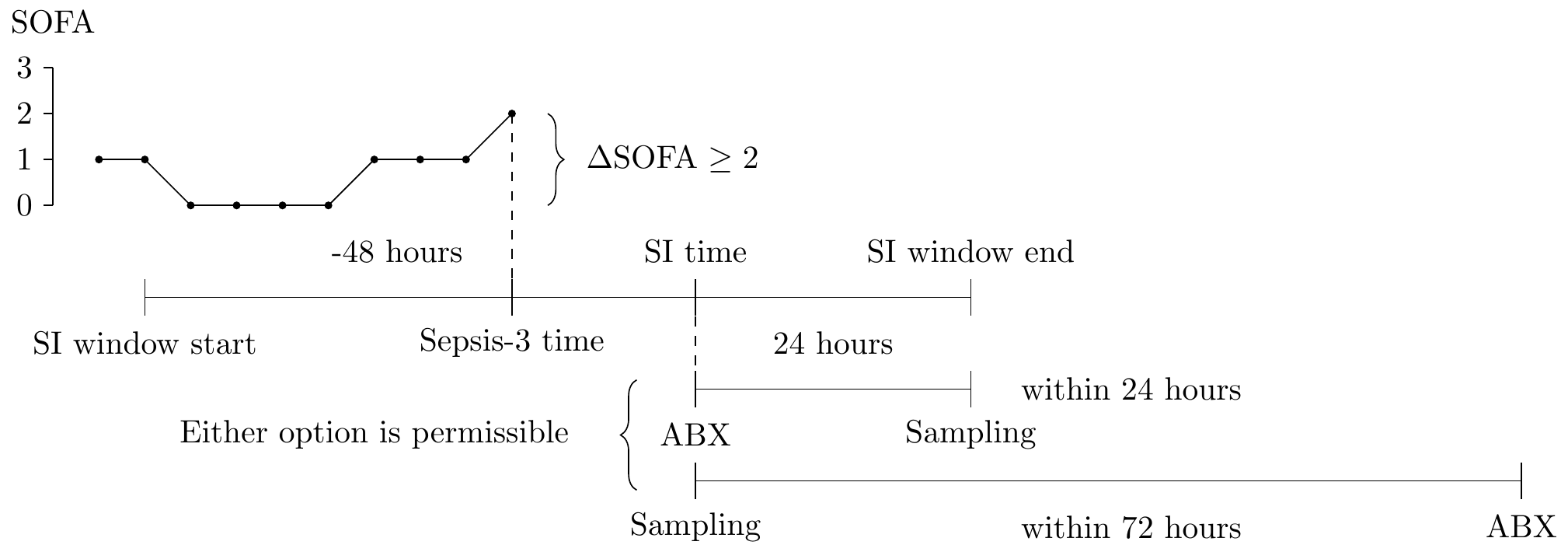
A patient can potentially have multiple SI windows. The argument
si_window is used to control which SI window we focus on (options are
"first", "last", "any").
Further, although a 2 or more point increase in the SOFA score is defined,
it is not perfectly clear to which value the increase refers. For this the
delta_fun argument is used. If the increase is required to happen with
respect to the minimal SOFA value (within the SI window) up to the current
time, the delta_cummin function should be used. If, however, we are
looking for an increase with respect to the start of the SI window, then
the delta_start function should be used. Lastly, the increase might be
defined with respect to values of the previous 24 hours, in which case the
delta_min function is used.
References
Singer M, Deutschman CS, Seymour CW, et al. The Third International Consensus Definitions for Sepsis and Septic Shock (Sepsis-3). JAMA. 2016;315(8):801–810. doi:10.1001/jama.2016.0287
Data setup
Description
Making a dataset available to ricu consists of 3 steps: downloading
(download_src()), importing (import_src()) and attaching
(attach_src()). While downloading and importing are one-time procedures,
attaching of the dataset is repeated every time the package is loaded.
Briefly, downloading loads the raw dataset from the internet (most likely
in .csv format), importing consists of some preprocessing to make the
data available more efficiently and attaching sets up the data for use by
the package. The download and import steps can be combined using
setup_src_data().
Usage
setup_src_data(x, ...)
Arguments
x |
Object specifying the source configuration |
... |
Forwarded to |
Details
If setup_src_data() is called on data sources that have all data available
with force = FALSE, nothing happens apart of a message being displayed. If
only a subset of tables is missing, only these tables are downloaded
(whenever possible) and imported. Passing force = TRUE attempts to re-
download and import the entire data set. If the data source is available
as a data package (as is the case for the two demo datasets), data is not
downloaded and imported, but this package is installed.
In most scenarios, setup_src_data() does not need to be called by users,
as upon package loading, all configured data sources are set up in a way
that enables download of missing data upon first access (and barring user
consent). However, instead of accessing all data sources where data
missingness should be resolved one by one, setup_src_data() is exported
for convenience.
Value
Called for side effects and returns NULL invisibly.
SIRS score label
Description
The SIRS (Systemic Inflammatory Response Syndrome) score is a commonly used assessment tool used to track a patient's well-being in an ICU.
Usage
sirs_score(
  ...,
  win_length = hours(24L),
  keep_components = FALSE,
  interval = NULL
)

qsofa_score(
  ...,
  win_length = hours(24L),
  keep_components = FALSE,
  interval = NULL
)

news_score(
  ...,
  win_length = hours(24L),
  keep_components = FALSE,
  interval = NULL
)

mews_score(
  ...,
  win_length = hours(24L),
  keep_components = FALSE,
  interval = NULL
)
Arguments
... |
Data input used for score evaluation |
win_length |
Window used for carry forward |
keep_components |
Logical flag indicating whether to return the individual components alongside the aggregated score |
interval |
Time series interval (only used for checking consistency of input data) |
SOFA score label
Description
The SOFA (Sequential Organ Failure Assessment) score is a commonly used
assessment tool for tracking a patient's status during a stay at an ICU.
Organ function is quantified by aggregating 6 individual scores,
representing respiratory, cardiovascular, hepatic, coagulation, renal and
neurological systems. The function sofa_score() is used as callback
function to the sofa concept but is exported as there are a few arguments
that can used to modify some aspects of the presented SOFA implementation.
Internally, sofa_score() calls first sofa_window(), followed by
sofa_compute() and arguments passed as ... will be forwarded to the
respective internally called function.
Usage
sofa_score(
  ...,
  worst_val_fun = max_or_na,
  explicit_wins = FALSE,
  win_length = hours(24L),
  keep_components = FALSE,
  interval = NULL
)

sofa_resp(..., interval = NULL)

sofa_coag(..., interval = NULL)

sofa_liver(..., interval = NULL)

sofa_cardio(..., interval = NULL)

sofa_cns(..., interval = NULL)

sofa_renal(..., interval = NULL)
Arguments
... |
Concept data, either passed as list or individual argument |
worst_val_fun |
functions used to calculate worst values over windows |
explicit_wins |
The default |
win_length |
Time-frame to look back and apply the |
keep_components |
Logical flag indicating whether to return the
individual components alongside the aggregated score (with a suffix |
interval |
Time series interval (only used for checking consistency
of input data, |
Details
The function sofa_score() calculates, for each component, the worst value
over a moving window as specified by win_length, using the function
passed as worst_val_fun. The default functions max_or_na() return NA
instead of -Inf/Inf in the case where no measurement is available over an
entire window. When calculating the overall score by summing up components
per time-step, a NA value is treated as 0.
Building on separate concepts, measurements for each component are converted to a component score using the definition by Vincent et. al.:
| SOFA score | 1 | 2 | 3 | 4 |
| Respiration | ||||
| PaO2/FiO2 [mmHg] | < 400 | < 300 | < 200 | < 100 |
| and mechanical ventilation | yes | yes | ||
| Coagulation | ||||
| Platelets [×103/mm3] | < 150 | < 100 | < 50 | < 20 |
| Liver | ||||
| Bilirubin [mg/dl] | 1.2-1.9 | 2.0-5.9 | 6.0-11.9 | > 12.0 |
| Cardiovasculara | ||||
| MAP | < 70 mmHg | |||
| or dopamine | ≤5 | > 5 | > 15 | |
| or dobutamine | any dose | |||
| or epinephrine | ≤0.1 | > 0.1 | ||
| or norepinephrine | ≤0.1 | > 0.1 | ||
| Central nervous system | ||||
| Glasgow Coma Score | 13-14 | 10-12 | 6-9 | < 6 |
| Renal | ||||
| Creatinine [mg/dl] | 1.2-1.9 | 2.0-3.4 | 3.5-4.9 | > 5.0 |
| or urine output [ml/day] | < 500 | < 200 | ||
Adrenergica agents administered for at least 1h (doses given are in [μg/kg · min]
At default, for each patient, a score is calculated for every time step,
from the first available measurement to the last. In instead of a regularly
evaluated score, only certain time points are of interest, this can be
specified using the explicit_wins argument: passing for example
hours(24, 48) will yield for every patient a score at hours 24 and 48
relative to the origin of the current ID system (for example ICU stay).
Value
A ts_tbl object.
References
Vincent, J.-L., Moreno, R., Takala, J. et al. The SOFA (Sepsis-related Organ Failure Assessment) score to describe organ dysfunction/failure. Intensive Care Med 22, 707–710 (1996). https://doi.org/10.1007/BF01709751
Stays
Description
Building on functionality offered by the (internal) function id_map(),
stay windows as well as (in case of differing values being passed as
id_type and win_type) an ID mapping is computed.
Usage
stay_windows(x, ...)

## S3 method for class 'src_env'
stay_windows(
  x,
  id_type = "icustay",
  win_type = id_type,
  in_time = "start",
  out_time = "end",
  interval = hours(1L),
  patient_ids = NULL,
  ...
)

## S3 method for class 'character'
stay_windows(x, ...)

## S3 method for class 'list'
stay_windows(x, ..., patient_ids = NULL)

## Default S3 method:
stay_windows(x, ...)
Arguments
x |
Data source (is coerced to |
... |
Generic consistency |
id_type |
Type of ID all returned times are relative to |
win_type |
Type of ID for which the in/out times is returned |
in_time, out_time |
column names of the returned in/out times |
interval |
The time interval used to discretize time stamps with,
specified as |
patient_ids |
Patient IDs used to subset the result |
Value
An id_tbl containing the selected IDs and depending on values
passed as in_time and out_time, start and end times of the ID passed as
win_var.
See Also
change_id
Suspicion of infection label
Description
Suspected infection is defined as co-occurrence of of antibiotic treatment and body-fluid sampling.
Usage
susp_inf(
  ...,
  abx_count_win = hours(24L),
  abx_min_count = 1L,
  positive_cultures = FALSE,
  si_mode = c("and", "or", "abx", "samp"),
  abx_win = hours(24L),
  samp_win = hours(72L),
  by_ref = TRUE,
  keep_components = FALSE,
  interval = NULL
)
Arguments
... |
Data and further arguments are passed to |
abx_count_win |
Time span during which to apply the |
abx_min_count |
Minimal number of antibiotic administrations |
positive_cultures |
Logical flag indicating whether to require cultures to be positive |
si_mode |
Switch between |
abx_win |
Time-span within which sampling has to occur |
samp_win |
Time-span within which antibiotic administration has to occur |
by_ref |
Logical flag indicating whether to process data by reference |
keep_components |
Logical flag indicating whether to return the individual components alongside the aggregated score |
interval |
Time series interval (only used for checking consistency of input data) |
Details
Suspected infection can occur in one of the two following ways:
administration of antibiotics followed by a culture sampling within
samp_winhoursabx_win |---------------| ABX sampling (last possible)
culture sampling followed by an antibiotic administration within
abx_winhourssamp_win |---------------------------------------------| sampling ABX (last possible)
The default values of samp_win and abx_win are 24 and 72 hours
respectively, as per Singer et.al. .
The earlier of the two times (fluid sampling, antibiotic treatment) is taken
as the time of suspected infection (SI time). The suspected infection
window (SI window) is defined to start si_lwr hours before the SI time
and end si_upr hours after the SI time. The default values of 48 and 24
hours (respectively) are chosen as used by Seymour et.al. (see
Supplemental Material).
                48h                       24h
  |------------------------------(|)---------------|
                                SI time
For some datasets, however, information on body fluid sampling is not
available for majority of the patients (eICU data). Therefore, an
alternative definition of suspected infection is required. For this, we use
administration of multiple antibiotics (argument abx_min_count determines
the required number) within abx_count_win hours. The first time of
antibiotic administration is taken as the SI time in this case.
References
Singer M, Deutschman CS, Seymour CW, et al. The Third International Consensus Definitions for Sepsis and Septic Shock (Sepsis-3). JAMA. 2016;315(8):801–810. doi:10.1001/jama.2016.0287
Seymour CW, Liu VX, Iwashyna TJ, et al. Assessment of Clinical Criteria for Sepsis: For the Third International Consensus Definitions for Sepsis and Septic Shock (Sepsis-3). JAMA. 2016;315(8):762–774. doi:10.1001/jama.2016.0288
Item callback utilities
Description
For concept loading, item callback functions are used in order to handle
item-specific post-processing steps, such as converting measurement units,
mapping a set of values to another or for more involved data
transformations, like turning absolute drug administration rates into rates
that are relative to body weight. Item callback functions are called by
load_concepts() with arguments x (the data), a variable number of name/
string pairs specifying roles of columns for the given item, followed by
env, the data source environment as src_env object.
Item callback functions can be specified by their name or using function
factories such as transform_fun(), apply_map() or convert_unit().
Usage
transform_fun(fun, ...)

binary_op(op, y)

comp_na(op, y)

set_val(val)

apply_map(map, var = "val_var")

convert_unit(fun, new, rgx = NULL, ignore_case = TRUE, ...)
Arguments
fun |
Function(s) used for transforming matching values |
... |
Further arguments passed to downstream function |
op |
Function taking two arguments, such as |
y |
Value passed as second argument to function |
val |
Value to replace every element of x with |
map |
Named atomic vector used for mapping a set of values (the names
of |
var |
Argument which is used to determine the column the mapping is applied to |
new |
Name(s) of transformed units |
rgx |
Regular expression(s) used for identifying observations based on
their current unit of measurement, |
ignore_case |
Forwarded to |
Details
The most forward setting is where a function is simply referred to by its name. For example in eICU, age is available as character vector due to ages 90 and above being represented by the string "> 89". A function such as the following turns this into a numeric vector, replacing occurrences of "> 89" by the number 90.
eicu_age <- function(x, val_var, ...) {
  data.table::set(
    data.table::set(x, which(x[[val_var]] == "> 89"), j = val_var,
                    value = 90),
    j = val_var,
    value = as.numeric(x[[val_var]])
  )
}
This function then is specified as item callback function for items
corresponding to eICU data sources of the age concept as
item(src = "eicu_demo", table = "patient", val_var = "age",
     callback = "eicu_age", class = "col_itm")
The string passed as callback argument is evaluated, meaning that an
expression can be passed which evaluates to a function that in turn can be
used as callback. Several function factories are provided which return
functions suitable for use as item callbacks: transform_fun() creates a
function that transforms the val_var column using the function supplied
as fun argument, apply_map() can be used to map one set of values to
another (again using the val_var column) and convert_unit() is intended
for converting a subset of rows (identified by matching rgx against the
unit_var column) by applying fun to the val_var column and setting
new as the transformed unit name (arguments are not limited to scalar
values). As transformations require unary functions, two utility function,
binary_op() and comp_na() are provided which can be used to fix the
second argument of binary functions such as * or ==. Taking all this
together, an item callback function for dividing the val_var column by 2
could be specified as "transform_fun(binary_op(/, 2))". The supplied
function factories create functions that operate on the data using
by-reference semantics. Furthermore, during concept
loading, progress is reported by a progress::progress_bar. In order to
signal a message without disrupting the current loading status, see
msg_progress().
Value
Callback function factories such as transform_fun(), apply_map()
or convert_unit() return functions suitable as item callback functions,
while transform function generators such as binary_op(), comp_na()
return functions that apply a transformation to a vector.
Examples
dat <- ts_tbl(x = rep(1:2, each = 5), y = hours(rep(1:5, 2)), z = 1:10)

subtract_3 <- transform_fun(binary_op(`-`, 3))
subtract_3(data.table::copy(dat), val_var = "z")

gte_4 <- transform_fun(comp_na(`>=`, 4))
gte_4(data.table::copy(dat), val_var = "z")

map_letters <- apply_map(setNames(letters[1:9], 1:9))
res <- map_letters(data.table::copy(dat), val_var = "z")
res

not_b <- transform_fun(comp_na(`!=`, "b"))
not_b(res, val_var = "z")
Internal utilities for ICU data objects
Description
In order to remove all id_tbl/ts_tbl-related attributes, as well as
extra class-labels, the exported but marked internal function
unclass_tbl() can be used. This function provides what one might expect
from an id_tbl/ts_tbl-specific implementation of the S3 generic
function data.table::as.data.table(). The inverse functionality if
provided by reclass_tbl() which attempts to add attributes as seen in
template to the object passed as x. The logical flag stop_on_fail
controls how to proceed if the attributes of template are incompatible
with the object x. Finally, in order to generate a template, as_ptype()
creates an empty object with the appropriate attributes.
Usage
unclass_tbl(x)

reclass_tbl(x, template, stop_on_fail = TRUE)

as_ptype(x)
Arguments
x |
Object to modify/query |
template |
Object after which to model the object in question |
stop_on_fail |
Logical flag indicating whether to consider failed object validation as error |
Value
-
unclass_tbl(): adata.table -
reclass_tbl(): either anid_tblor ats_tbldepending on the type of the object passed astemplate -
as_ptype(): an object of the same type asx, but with on data
Read and write utilities
Description
Support for reading from and writing to pipe separated values (.psv)
files as used for the PhysioNet Sepsis Challenge.
Usage
write_psv(x, dir, na_rows = NULL)

read_psv(dir, col_spec = NULL, id_var = "stay_id", index_var = NULL)
Arguments
x |
Object to write to files |
dir |
Directory to write the (many) files to or read from |
na_rows |
If |
col_spec |
A column specification as created by |
id_var |
Name of the id column (IDs are generated from file names) |
index_var |
Optional name of index column (will be coerced to
|
Details
Data for the PhysioNet Sepsis Challenge is distributed as pipe separated
values (.psv) files, split into separate files per patient ID, containing
time stamped rows with measured variables as columns. Files are named with
patient IDs and do not contain any patient identifiers as data. Functions
read_psv() and write_psv() can be used to read from and write to such
a data format.
Value
While write_psv() is called for side effects and returns NULL
invisibly, read_psv() returns an object inheriting from id_tbl.
References
Reyna, M., Josef, C., Jeter, R., Shashikumar, S., Moody, B., Westover, M. B., Sharma, A., Nemati, S., & Clifford, G. (2019). Early Prediction of Sepsis from Clinical Data – the PhysioNet Computing in Cardiology Challenge 2019 (version 1.0.0). PhysioNet. https://doi.org/10.13026/v64v-d857.