| Title: | Just Analysis Methods Base |
| Version: | 1.0.4 |
| Description: | Just analysis methods ('jam') base functions focused on bioinformatics. Version- and gene-centric alphanumeric sort, unique name and version assignment, colorized console and 'HTML' output, color ramp and palette manipulation, 'Rmarkdown' cache import, styled 'Excel' worksheet import and export, interpolated raster output from smooth scatter and image plots, list to delimited vector, efficient list tools. |
| Depends: | R (≥ 3.0.0) |
| Imports: | methods, grDevices, graphics, stats, utils, colorspace, RColorBrewer, KernSmooth, withr |
| Suggests: | crayon, farver, knitr, rmarkdown, testthat (≥ 3.0.0) |
| Enhances: | ggplot2, ggridges, IRanges, S4Vectors, openxlsx, kableExtra, matrixStats, viridisLite, ComplexHeatmap, circlize, GenomicRanges, igraph, pryr, rstudioapi, Matrix, sparseMatrixStats |
| License: | MIT + file LICENSE |
| Encoding: | UTF-8 |
| URL: | https://jmw86069.github.io/jamba/ |
| BugReports: | https://github.com/jmw86069/jamba/issues |
| VignetteBuilder: | knitr |
| RoxygenNote: | 7.3.2 |
| Config/testthat/edition: | 3 |
| NeedsCompilation: | no |
| Packaged: | 2025-03-23 06:31:56 UTC; wardjm |
| Author: | James M. Ward  [aut, cre, cph]
 |
| Maintainer: | James M. Ward <jmw86069@gmail.com> |
| Repository: | CRAN |
| Date/Publication: | 2025-03-23 16:30:02 UTC |
jamba: Jam Base Methods
Description
The jamba package contains several jam base functions which are re-usable for routine R analysis work, and are important dependencies for other Jam R packages.
Details
See the function reference for a complete list of functions.
The goal is to implement methods as lightweight as possible, so so inclusion in an analysis workflow will not incur a noticeable burden.
plot functions
-
plotSmoothScatter()smoothScatter() enhanced for more visual detail -
imageDefault()enhanced rasterized image() with fixed aspect ratio -
imageByColors()fordata.frameof colors and optional labels centered across repeated values. -
showColors()color display for vector, list, color function, or mixed formats. -
nullPlot()blank plot that labels the current margin sizes -
minorLogTicksAxis()log-scale axis ticks in base R with custom log base, optional offset, e.g.log2(1 + x) -
shadowText()base R text labels with shadow or outline or both, alsoshadowText_options(). -
getPlotAspect(),decideMfrow()convenience base R graphics.
string functions
-
mixedSort(),mixedOrder(),mixedSortDF()- efficient alphanumeric "version" sort, with options helpful for gene symbols. -
vgrep(),vigrep(),igrep(),vigrep()fast grep wrappers for value-return, case-insensitive search. -
provigrep(),proigrep()- progressive, ordered grep to use pattern matching to re-order a vector. -
makeNames()create unique, versioned names with custom format -
nameVector()apply names to vector dynamically -
nameVectorN()vector of named names useful withlapply(). -
pasteByRow(),pasteByRowOrdered()paste data.frame and matrix values by row, skipping blanks, optional factor order. -
rbindList()convert list tomatrixordata.frame. -
tcount()extendstable()to sort by size and optional minimum count filter.
color functions
-
rgb2col(),col2hcl(),col2hcl(),col2hsv(),hsv2col()color interconversion -
setTextContrastColor()text contrast color per given background color -
getColorRamp()catch-all to get named gradients, or expand one or more colors to gradient. -
makeColorDarker(),color2gradient(),showColors()color manipulation and display
miscellaneous helper functions
-
printDebug()colored text output to console, 'Rmarkdown', HTML -
kable_coloring()coloredkableExtra::kable()output for 'Rmarkdown' -
setPrompt()colored R prompt -
getDate(),asDate(),dateToDaysOld()human-readable, opinionated date formatting -
padString(),padInteger()pad character or integer strings -
rmNA(),rmNULL(),rmInfinite()remove or replace missing or NA values with defined alternatives
export and import functions
-
readOpenxlsx()import worksheets from 'xlsx' 'Excel' files. -
writeOpenxlsx()export worksheets to 'xlsx' 'Excel' files with color, formatting, and styling.
Jam options
The jamba package recognizes some global options, but limits these
options to include only non-analysis options. For example, no global
option should change the numerical manipulation of data.
-
jam.lightMode-logicalwhether the R console or graphical background is light or dark,printDebug()limits the luminance range to maximize visual contrast. -
jam.Crange,jam.Lrange- numerical values used byprintDebug()to maximize visual contrast, used withjam.lightMode. -
jam.shadowColor,jam.shadow.r,jam.shadow.n,jam.alphaShadow,jam.outline,jam.alphaOutlineto customize details forshadowText(), seeshadowText_options()for convenience.
Author(s)
Maintainer: James M. Ward jmw86069@gmail.com (ORCID) [copyright holder]
See Also
Useful links:
Adjust axis label margins
Description
Adjust axis label margins to accommodate axis labels
Usage
adjustAxisLabelMargins(
  x,
  margin = 1,
  maxFig = 1/2,
  cex = graphics::par("cex"),
  cex.axis = graphics::par("cex.axis"),
  prefix = "-- -- ",
  ...
)
Arguments
x |
|
margin |
|
maxFig |
|
cex |
|
cex.axis |
|
prefix |
|
... |
additional parameters are ignored. |
Details
This function takes a vector of axis labels, and the margin where they
will be used, and adjusts the relevant axis margin to accomodate the
label size, up to a maximum fraction of the figure size as defined by
maxFig.
Labels are assumed to be perpendicular to the axis, for example
argument las=2 when using graphics::text().
Note this function does not render labels in the figure, and therefore does not revert axis margins to their original size. That process should be performed separately.
Value
list named "mai" suitable for use in graphics::par()
to adjust margin size using in inches.
See Also
Other jam plot functions:
coordPresets(),
decideMfrow(),
drawLabels(),
getPlotAspect(),
groupedAxis(),
imageByColors(),
imageDefault(),
minorLogTicksAxis(),
nullPlot(),
plotPolygonDensity(),
plotRidges(),
plotSmoothScatter(),
shadowText(),
shadowText_options(),
showColors(),
sqrtAxis(),
usrBox()
Examples
xlabs <- paste0("item_", (1:20));
ylabs <- paste0("rownum_", (1:20));

# proper adjustment should be done using withr, for example
x_cex <- 0.8;
y_cex <- 1.2;
withr::with_par(adjustAxisLabelMargins(xlabs, 1, cex.axis=x_cex), {
   withr::local_par(adjustAxisLabelMargins(ylabs, 2, cex.axis=y_cex))
   nullPlot(xlim=c(1,20), ylim=c(1,20), doMargins=FALSE);
   graphics::axis(1, at=1:20, labels=xlabs, las=2, cex.axis=x_cex);
   graphics::axis(2, at=1:20, labels=ylabs, las=2, cex.axis=y_cex);
})

withr::with_par(adjustAxisLabelMargins(xlabs, 3, cex.axis=x_cex), {
   withr::local_par(adjustAxisLabelMargins(ylabs, 4, cex.axis=y_cex))
   nullPlot(xlim=c(1,20), ylim=c(1,20), doMargins=FALSE);
   graphics::axis(3, at=1:20, labels=xlabs, las=2);
   graphics::axis(4, at=1:20, labels=ylabs, las=2);
})

par("mar")
set R color alpha value
Description
Define the alpha transparency per R color
Usage
alpha2col(x, alpha = 1, maxValue = 1, ...)
Arguments
x |
R compatible color, either a color name, or hex value, or
a mixture of the two. Any value compatible with |
alpha |
numeric alpha transparency to use per x color. alpha is recycled to length(x) as needed. |
maxValue |
numeric maximum value to return, useful when the downstream alpha range should be 255. By default maxValue=1 is returned. |
... |
Additional arguments are ignored. |
Value
character vector of R colors, with alpha values.
See Also
Other jam color functions:
applyCLrange(),
col2alpha(),
col2hcl(),
col2hsl(),
col2hsv(),
color2gradient(),
fixYellow(),
fixYellowHue(),
getColorRamp(),
hcl2col(),
hsl2col(),
hsv2col(),
isColor(),
kable_coloring(),
makeColorDarker(),
rainbow2(),
rgb2col(),
setCLranges(),
setTextContrastColor(),
showColors(),
unalpha(),
warpRamp()
Examples
withr::with_par(list("mfrow"=c(2,2)), {
for (alpha in c(1, 0.8, 0.5, 0.2)) {
   nullPlot(plotAreaTitle=paste0("alpha=", alpha),
      doMargins=FALSE);
   usrBox(fill=alpha2col("yellow",
      alpha=alpha));
}
})
Apply CL color range
Description
Restrict chroma (C) and luminance (L) ranges for a vector of R colors
Usage
applyCLrange(
  x,
  lightMode = NULL,
  Crange = getOption("jam.Crange"),
  Lrange = getOption("jam.Lrange"),
  Cgrey = getOption("jam.Cgrey", 5),
  fixYellow = TRUE,
  CLmethod = c("scale", "floor", "expand"),
  fixup = TRUE,
  ...
)
Arguments
x |
vector of R colors |
lightMode |
|
Crange |
|
Lrange |
|
Cgrey |
|
fixYellow |
|
CLmethod |
|
fixup |
|
... |
additional argyments are passed to |
Details
This function is primarily intended to restrict the range of brightness values so they contrast with a background color, particularly when the background color may be bright or dark.
Note that output is slightly different when supplying one color,
compared to supplying a vector of colors. One color is simply
restricted to the Crange and Lrange. However, a vector of colors
is scaled within the ranges so that relative C and L values
are maintained, for visual comparison.
The C and L values are defined by colorspace::polarLUV(), where C is
typically restricted to 0..100 and L is typically 0..100. For some
colors, values above 100 are allowed.
Values are restricted to the given numeric range using one of three
methods, set via the CLmethod argument.
As an example, consider what should be done when Crange <- c(10,70)
and the C values are Cvalues <- c(50, 60, 70, 80).
"floor" uses
jamba::noiseFloor()to apply fixed cutoffs at the minimum and maximum range. This method has the effect of making all values outside the range into an equal final value."scale" will apply
jamba::normScale()to rescale only values outside the given range. For example,c(Crange, Cvalues)as the initial range, it constrains values toc(Crange). This method has the effect of maintaining the relative difference between values."expand" will simply apply
jamba::normScale()to fit the values to the minimum and maximum range values. This method has the effect of forcing colors to fit the full numeric range, even when the original differences between values were small.
In case (1) above, Cvalues will become c(50, 60, 70, 70).
In case (2) above, Cvalues will become c(44, 53, 61, 70)
In case (3) above, Cvalues will become c(10, 30, 50, 70)
Note that colors with C (chroma) values less than Cgrey will not have
the C value changed, in order to maintain colors at a greyscale, without
colorizing them. Particularly for pure grey, which has C=0, but
is still required to have a hue H, it is important not to increase
C.
Value
vector of colors after applying the chroma (C) and luminance (L) ranges.
See Also
Other jam color functions:
alpha2col(),
col2alpha(),
col2hcl(),
col2hsl(),
col2hsv(),
color2gradient(),
fixYellow(),
fixYellowHue(),
getColorRamp(),
hcl2col(),
hsl2col(),
hsv2col(),
isColor(),
kable_coloring(),
makeColorDarker(),
rainbow2(),
rgb2col(),
setCLranges(),
setTextContrastColor(),
showColors(),
unalpha(),
warpRamp()
Examples
cl <- c("red", "blue", "navy", "yellow", "orange");
cl_lite <- applyCLrange(cl, lightMode=TRUE);
cl_dark <- applyCLrange(cl, lightMode=FALSE);

# individual colors
cl_lite_ind <- sapply(cl, applyCLrange, lightMode=TRUE);
cl_dark_ind <- sapply(cl, applyCLrange, lightMode=FALSE);

# display colors
showColors(list(`input colors`=cl,
   `lightMode=TRUE, vector`=cl_lite,
   `lightMode=TRUE, individual`=cl_lite_ind,
   `lightMode=FALSE, vector`=cl_dark,
   `lightMode=FALSE, individual`=cl_dark_ind))
printDebug(cl, lightMode=TRUE);
Add categorical colors to 'Excel' 'xlsx' worksheets
Description
Add categorical colors to 'Excel' 'xlsx' worksheets
Usage
applyXlsxCategoricalFormat(
  xlsxFile,
  sheet = 1,
  rowRange = NULL,
  colRange = NULL,
  colorSub = NULL,
  colorSubText = setTextContrastColor(colorSub),
  trimCatNames = TRUE,
  overwrite = TRUE,
  wrapText = FALSE,
  stack = TRUE,
  verbose = FALSE,
  ...
)
Arguments
xlsxFile |
|
sheet |
|
rowRange, colRange |
|
colorSub |
one of the following types of input:
|
colorSubText |
optional |
trimCatNames |
|
overwrite |
|
wrapText |
|
stack |
|
verbose |
|
... |
additional arguments are ignored. |
Details
This function is a convenient wrapper for applying categorical
color formatting to cell background colors, and applies a contrasting
color to the text in cells using setTextContrastColor().
It uses a named character vector of colors supplied as colorSub
to define cell background colors, and optionally colorSubText
to define a specific color for the cell text.
Value
Workbook object as defined by the openxlsx package
is returned invisibly with invisible(). This Workbook
can be used in argument wb to provide a speed boost when
saving multiple sheets to the same file.
See Also
Other jam export functions:
applyXlsxConditionalFormat(),
readOpenxlsx(),
set_xlsx_colwidths(),
set_xlsx_rowheights(),
writeOpenxlsx()
Examples
# write to tempfile for examples
if (check_pkg_installed("openxlsx")) {
   out_xlsx <- tempfile(pattern="writeOpenxlsx_", fileext=".xlsx")
   df <- data.frame(a=LETTERS[1:5], b=1:5);
   writeOpenxlsx(x=df,
      file=out_xlsx,
      sheetName="jamba_test");

   colorSub <- nameVector(
      rainbow2(5, s=c(0.8, 1), v=c(0.8, 1)),
      LETTERS[1:5]);
   applyXlsxCategoricalFormat(out_xlsx,
      sheet="jamba_test",
      colorSub=colorSub
   )
}
Xlsx Conditional formatting
Description
Xlsx Conditional formatting
Usage
applyXlsxConditionalFormat(
  xlsxFile,
  sheet = 1,
  fcColumns = NULL,
  fcGrep = NULL,
  fcStyle = c("#4F81BD", "#EEECE1", "#C0504D"),
  fcRule = c(-6, 0, 6),
  fcType = "colourScale",
  lfcColumns = NULL,
  lfcGrep = NULL,
  lfcStyle = c("#4F81BD", "#EEECE1", "#C0504D"),
  lfcRule = c(-3, 0, 3),
  lfcType = "colourScale",
  hitColumns = NULL,
  hitGrep = NULL,
  hitStyle = c("#4F81BD", "#EEECE1", "#C0504D"),
  hitRule = c(-1.5, 0, 1.5),
  hitType = "colourScale",
  intColumns = NULL,
  intGrep = NULL,
  intStyle = c("#EEECE1", "#FDC99B", "#F77F30"),
  intRule = c(0, 100, 10000),
  intType = "colourScale",
  numColumns = NULL,
  numGrep = NULL,
  numStyle = c("#F2F0F7", "#B4B1D4", "#938EC2"),
  numRule = c(1, 10, 20),
  numType = "colourScale",
  pvalueColumns = NULL,
  pvalueGrep = NULL,
  pvalueStyle = c("#F77F30", "#FDC99B", "#EEECE1"),
  pvalueRule = c(0, 0.01, 0.05),
  pvalueType = "colourScale",
  verbose = FALSE,
  startRow = 2,
  overwrite = TRUE,
  ...
)
Arguments
xlsxFile |
|
sheet |
integer or character, either the worksheet number, in order or character worksheet name. This vector can contain multiple values, which will cause conditional formatting to be applied to each worksheet in the order given. |
fcColumns, lfcColumns, hitColumns, intColumns, numColumns, pvalueColumns |
integer column indices, or character colnames indicating which columns are to be treated as each of the various column types. |
fcGrep, lfcGrep, hitGrep, intGrep, numGrep, pvalueGrep |
optional character vector which is used by |
fcStyle, lfcStyle, hitStyle, intStyle, numStyle, pvalueStyle |
color vector of length=3, corresponding to the numeric thresholds defined by the corresponding Rules. |
fcRule, lfcRule, hitRule, intRule, numRule, pvalueRule |
numeric vector of length=3, used to define three numeric thresholds for color gradients to be applied. |
fcType, lfcType, hitType, intType, numType, pvalueType |
character string indicating the type of conditional rule to apply,
which in most cases should be "colourScale" which allows three numeric
thresholds, and three corresponding colors. For other allowed values,
see |
verbose |
logical indicating whether to print verbose output. |
startRow |
integer indicating which row to begin applying conditional formatting. In most cases startRow=2, which allows one row for column headers. However, if there are multiple header rows, startRow should be 1 more than the number of header rows. |
overwrite |
logical indicating whether the original 'Excel' files will be replaced with the new one, or whether a new file will be created. |
... |
additional parameters are ignored. |
Details
This function is a convenient wrapper for applying conditional formatting to 'Excel' 'xlsx' worksheets, with reasonable settings for commonly used data types.
Note that this function does not apply cell formatting, such as numeric formatting as displayed in 'Excel'.
A description of column types follows:
- "fc"
Fold change, typically positive and negative values, which are formatted to show one decimal place, and use commas to separate thousands places, e.g. 1,020.1. Colors are applied with a neutral midpoint, coloring values which are above and below zero.
- "lfc"
log fold change, typically positive and negative values, which are formatted to show one decimal place, and use commas to separate thousands places, e.g. 12.1. Colors are applied with a neutral midpoint, coloring values which are above and below zero. Log fold changes have slightly different color thresholds than fold changes.
- "hit"
Hit columns, often just values like
c(-1,0,1), but which could be fold changes for statistical hits for example. They are formatted to show one decimal place, and use commas to separate thousands places, e.g. 1.5. Colors are applied with a neutral midpoint, coloring values which are above and below zero, typically with a fairly low threshold.- "int"
Integer columns, which are formatted to hide decimal place values even if present, which can help clean up visible tabular data. They are formatted to use commas to separate thousands places, e.g. 1,020. Colors are applied with a baseline of zero, intended for highlighting two thresholds of values above zero.
- "num"
Numeric columns, which are formatted to display 2 decimal places, and to use commas to separate thousands places, e.g. 1,020.1. Colors are applied with a baseline of zero, intended for highlighting two thresholds of values above zero.
- "pvalue"
P-value columns, which are formatted to display scientific notation always, for consistency, with two decimal places, e.g. 1.02e-02. Colors are applied starting at white for P-value of 1 (non-significant) and becoming more red as the P-value approaches 0.01, then 0.0001.
For each column type, one can describe the column using integer indices,
or colnames, or optionally use the Grep parameters. The Grep parameters
are intended for pattern matching, and may contain a vector of grep patterns
which are used by provigrep() to match to colnames. The Grep
method is particularly useful when applying conditional formatting for
multiple worksheets in the same 'xlsx' file, where the colnames are not
identical in each worksheet.
Each column type has an associated 3-threshold rule, and three associated colors. In order to apply different thresholds, one would need to call this function multiple times, specifying different subsets of columns corresponding to each set of thresholds. The same process is required in order to apply different color gradients to different columns. Note that styles are by default "stacked", which maintains font and cell border styles without removing them. However, it this "stacking" means that applying two rules to the same cell will not work, since only the first rule will be applied by 'Microsoft Excel'. Interestingly, if multiple conditional rules are applied to the same cell, they will be visible in order inside the 'Microsoft Excel' application.
Value
Workbook object as defined by the openxlsx package
is returned invisibly with invisible(). This Workbook
can be used in argument wb to provide a speed boost when
saving multiple sheets to the same file.
See Also
Other jam export functions:
applyXlsxCategoricalFormat(),
readOpenxlsx(),
set_xlsx_colwidths(),
set_xlsx_rowheights(),
writeOpenxlsx()
Examples
# write to tempfile for examples
if (check_pkg_installed("openxlsx")) {
   out_xlsx <- tempfile(pattern="writeOpenxlsx_", fileext=".xlsx")
   df <- data.frame(a=LETTERS[1:5], b=1:5);
   writeOpenxlsx(x=df,
      file=out_xlsx,
      sheetName="jamba_test");

   applyXlsxConditionalFormat(out_xlsx,
      sheet="jamba_test",
      intColumns=2,
      intRule=c(0,3,5),
      intStyle=c("#FFFFFF", "#1E90FF", "#9932CC")
   )
}
convert date DDmmmYYYY to Date
Description
convert date DDmmmYYYY to Date
Usage
asDate(getDateValues, dateFormat = "%d%b%Y", ...)
Arguments
getDateValues |
|
dateFormat |
|
... |
additional parameters are ignored. |
Details
This function converts a text date string to Date object, mainly to
allow date-related math operations, for example difftime.
Value
Date object
See Also
Other jam date functions:
dateToDaysOld(),
getDate()
Examples
asDate(getDate());
convert numeric value or R object to human-readable size
Description
convert numeric value or R object to human-readable size
Usage
asSize(
  x,
  digits = 3,
  abbreviateUnits = TRUE,
  unitType = "bytes",
  unitAbbrev = gsub("^(.).*$", "\\1", unitType),
  kiloSize = 1024,
  sep = " ",
  ...
)
Arguments
x |
|
digits |
|
abbreviateUnits |
|
unitType |
|
unitAbbrev |
|
kiloSize |
|
sep |
|
... |
other parameters passed to |
Details
This function returns human-readable size based upon numeric input.
Alternatively, when input is any other R object, it calls
utils::object.size() to produce a single numeric value which is then
used to produce human-readable size.
The default behavior is to report computer size in bytes, where
1024 is considered "kilo", however argument kiloSize can be
used to produce values where kiloSize=1000 which is suitable
for monetary and other scientific values.
Value
character vector representing human-friendly size,
based upon the kiloSize argument to determine whether to
report byte (1024) or scientific (1000) units.
See Also
Other jam string functions:
breaksByVector(),
fillBlanks(),
formatInt(),
gsubOrdered(),
gsubs(),
makeNames(),
nameVector(),
nameVectorN(),
padInteger(),
padString(),
pasteByRow(),
pasteByRowOrdered(),
sizeAsNum(),
tcount(),
ucfirst()
Examples
asSize(c(1, 10,2010,22000,52200))
#> "1 byte"   "10 bytes" "2 kb"     "21 kb"    "51 kb"

# demonstration of straight numeric units
asSize(c(1, 100, 1000, 10000), unitType="", kiloSize=100)
Calculate more detailed density of numeric values
Description
Calculate more detailed density of numeric values
Usage
breakDensity(
  x,
  breaks = length(x)/3,
  bw = NULL,
  width = NULL,
  densityBreaksFactor = 3,
  weightFactor = 1,
  addZeroEnds = TRUE,
  baseline = 0,
  floorBaseline = FALSE,
  verbose = FALSE,
  ...
)
Arguments
x |
numeric vector |
breaks |
numeric breaks as described for |
bw |
character name of a bandwidth function, or NULL. |
width |
NULL or numeric value indicating the width of breaks to apply. |
densityBreaksFactor |
numeric factor to adjust the width of density breaks, where higher values result in less detail. |
weightFactor |
optional vector of weights |
addZeroEnds |
logical indicating whether the start and end value should always be zero, which can be helpful for creating a polygon. |
baseline |
optional numeric value indicating the expected baseline, which is typically zero, but can be set to a higher value to indicate a "noise floor". |
floorBaseline |
logical indicating whether to apply a noise floor to the output data. |
verbose |
logical indicating whether to print verbose output. |
... |
additional parameters are sent to |
Details
This function is a drop-in replacement for stats::density(),
simply to provide a quick alternative that defaults to a higher
level of detail. Detail can be adjusted using densityBreaksFactor,
where higher values will use a wider step size, thus lowering
the detail in the output.
Note that the density height is scaled by the total number of points,
and can be adjusted with weightFactor. See Examples for how to
scale the y-axis range similar to stats::density().
Value
list output equivalent to stats::density():
-
x: Thencoordinates of the points where the density is estimated. -
y: The estimated density values, non-negative, but can be zero. -
bw: The bandidth used. -
n: The sample size after elimination of missing values. -
call: the call which produced the result. -
data.name: the deparsed name of thexargument. -
has.na:logicalfor compatibility, and alwaysFALSE.
See Also
Other jam practical functions:
call_fn_ellipsis(),
checkLightMode(),
check_pkg_installed(),
colNum2excelName(),
color_dither(),
exp2signed(),
getAxisLabel(),
isFALSEV(),
isTRUEV(),
jargs(),
kable_coloring(),
lldf(),
log2signed(),
middle(),
minorLogTicks(),
newestFile(),
printDebug(),
reload_rmarkdown_cache(),
renameColumn(),
rmInfinite(),
rmNA(),
rmNAs(),
rmNULL(),
setPrompt()
Examples
x <- c(stats::rnorm(15000),
   stats::rnorm(5500)*0.25 + 1,
   stats::rnorm(12500)*0.5 + 2.5)
plot(stats::density(x))

plot(breakDensity(x))

plot(breakDensity(x, densityBreaksFactor=200))

# trim values to show abrupt transitions
x2 <- x[x > 0 & x < 4]
plot(stats::density(x2), lwd=2)
lines(breakDensity(x2, weightFactor=1/length(x2)/10), col="red")
graphics::legend("topright", c("stats::density()", "breakDensity()"),
   col=c("black", "red"), lwd=c(2, 1))
break a vector into groups
Description
breaks a vector into groups
Usage
breaksByVector(x, labels = NULL, returnFractions = FALSE, ...)
Arguments
x |
|
labels |
|
returnFractions |
|
... |
additional parameters are ignored. |
Details
This function takes a vector of values, determines "chunks" of identical values, from which it defines where breaks occur. It assumes the input vector is ordered in the way it will be displayed, with some labels being duplicated consecutively. This function defines the breakpoints where the labels change, and returns the ideal position to put a single label to represent a duplicated consecutive set of labels.
It can return fractional coordinates, for example when a label represents two consecutive items, the fractional coordinate can be used to place the label between the two items.
This function is useful for things like adding labels to
imageDefault() color image map of sample groupings, where
it may be ideal to label only unique elements in a contiguous set.
Value
list with the following named elements:
-
"breakPoints": The mid-point coordinate between each break. These midpoints would be good for drawing dividing lines for example. -
"labelPoints": The ideal point to place a label to represent the group. -
"newLabels": A vector of labels the same length as the input data, except using blank values except where a label should be drawn. This output is good for text display. -
"useLabels": The unique set of labels, without blanks, corresponding to the coordinates supplied by labelPoints. -
"breakLengths": The integer size of each set of labels.
See Also
Other jam string functions:
asSize(),
fillBlanks(),
formatInt(),
gsubOrdered(),
gsubs(),
makeNames(),
nameVector(),
nameVectorN(),
padInteger(),
padString(),
pasteByRow(),
pasteByRowOrdered(),
sizeAsNum(),
tcount(),
ucfirst()
Examples
b <- rep(LETTERS[c(1:5, 1)], c(2,3,5,4,3,4));
bb <- breaksByVector(b);
# Example showing how labels can be minimized inside a data.frame
data.frame(b,
   newLabels=bb$newLabels);

# Example showing how to reposition text labels
# so duplicated labels are displayed in the middle
# of each group
bb2 <- breaksByVector(b, returnFractions=TRUE);
ylabs <- c("minimal labels", "all labels");
withr::with_par(adjustAxisLabelMargins(ylabs, 2), {
   withr::local_par(adjustAxisLabelMargins(bb2$useLabels, 1))
   nullPlot(xlim=range(seq_along(b)), ylim=c(0,3),
      doBoxes=FALSE, doUsrBox=TRUE);
   graphics::axis(2, las=2, at=c(1,2), ylabs);
   graphics::text(y=2, x=seq_along(b), b);
   graphics::text(y=1, x=bb2$labelPoints, bb2$useLabels);

## Print axis labels in the center of each group
graphics::axis(3,
   las=2,
   at=bb2$labelPoints,
   labels=bb2$useLabels);

## indicate each region
for (i in seq_along(bb2$breakPoints)) {
   graphics::axis(1,
      at=c(c(0, bb2$breakPoints)[i]+0.8, bb2$breakPoints[i]+0.2),
      labels=c("", ""));
}
## place the label centered in each region without adding tick marks
graphics::axis(1,
   las=2,
   tick=FALSE,
   at=bb2$labelPoints,
   labels=bb2$useLabels);
## abline to indicate the boundaries, if needed
graphics::abline(v=c(0, bb2$breakPoints) + 0.5,
   lty="dashed",
   col="blue");

})
# The same process is used by imageByColors()
paste a list into a delimited vector
Description
Paste a list of vectors into a character vector, with values delimited by default with a comma.
Usage
cPaste(
  x,
  sep = ",",
  doSort = FALSE,
  makeUnique = FALSE,
  na.rm = FALSE,
  keepFactors = FALSE,
  checkClass = TRUE,
  useBioc = TRUE,
  useLegacy = FALSE,
  honorFactor = TRUE,
  verbose = FALSE,
  ...
)

cPasteS(
  x,
  sep = ",",
  doSort = TRUE,
  makeUnique = FALSE,
  na.rm = FALSE,
  keepFactors = FALSE,
  checkClass = TRUE,
  useBioc = TRUE,
  ...
)

cPasteSU(
  x,
  sep = ",",
  doSort = TRUE,
  makeUnique = TRUE,
  na.rm = FALSE,
  keepFactors = FALSE,
  checkClass = TRUE,
  useBioc = TRUE,
  ...
)

cPasteUnique(
  x,
  sep = ",",
  doSort = FALSE,
  makeUnique = TRUE,
  na.rm = FALSE,
  keepFactors = FALSE,
  checkClass = TRUE,
  useBioc = TRUE,
  ...
)

cPasteU(
  x,
  sep = ",",
  doSort = FALSE,
  makeUnique = TRUE,
  na.rm = FALSE,
  keepFactors = FALSE,
  checkClass = TRUE,
  useBioc = TRUE,
  ...
)
Arguments
x |
|
sep |
|
doSort |
|
makeUnique |
|
na.rm |
|
keepFactors |
|
checkClass |
|
useBioc |
|
useLegacy |
|
honorFactor |
|
verbose |
|
... |
additional arguments are passed to |
Details
-
cPaste()concatenates vector values using a delimiter. -
cPasteS()sorts each vector usingmixedSort(). -
cPasteU()appliesuniques()to retain unique values per vector. -
cPasteSU()appliesmixedSort()anduniques().
This function is essentially a wrapper for S4Vectors::unstrsplit()
except that it also optionally applies uniqueness to each vector
in the list, and sorts values in each vector using mixedOrder().
The sorting and uniqueness is applied to the unlisted vector of
values, which is substantially faster than any apply family function
equivalent. The uniqueness is performed by uniques(), which itself
will use S4Vectors::unique() if available.
Value
character vector with the same names and in the same order
as the input list x.
See Also
Other jam list functions:
heads(),
jam_rapply(),
list2df(),
mergeAllXY(),
mixedSorts(),
rbindList(),
relist_named(),
rlengths(),
sclass(),
sdim(),
uniques(),
unnestList()
Examples
L1 <- list(CA=LETTERS[c(1:4,2,7,4,6)], B=letters[c(7:11,9,3)]);

cPaste(L1);
#               CA                 B
# "A,B,C,D,B,G,D,F"   "g,h,i,j,k,i,c"

cPaste(L1, doSort=TRUE);
#               CA                 B
# "A,B,B,C,D,D,F,G"   "c,g,h,i,i,j,k"

## The sort can be done with convenience function cPasteS()
cPasteS(L1);
#               CA                 B
# "A,B,B,C,D,D,F,G"   "c,g,h,i,i,j,k"

## Similarly, makeUnique=TRUE and cPasteU() are the same
cPaste(L1, makeUnique=TRUE);
cPasteU(L1);
#           CA             B
# "A,B,C,D,G,F" "g,h,i,j,k,c"

## Change the delimiter
cPasteSU(L1, sep="; ")
#                CA                  B
# "A; B; C; D; F; G" "c; g; h; i; j; k"

# test mix of factor and non-factor
L2 <- c(
   list(D=factor(letters[1:12],
      levels=letters[12:1])),
   L1);
L2;
cPasteSU(L2, keepFactors=TRUE);

# tricky example with mix of character and factor
# and factor levels are inconsistent
# end result: factor levels are defined in order they appear
L <- list(entryA=c("miR-112", "miR-12", "miR-112"),
   entryB=factor(c("A","B","A","B"),
      levels=c("B","A")),
   entryC=factor(c("C","A","B","B","C"),
      levels=c("A","B","C")),
   entryNULL=NULL)
L;
cPaste(L);
cPasteU(L);

# by default keepFactors=FALSE, which means factors are sorted as characters
cPasteS(L);
cPasteSU(L);
# keepFactors=TRUE will keep unique factor levels in the order they appear
# this is the same behavior as unlist(L[c(2,3)]) on a list of factors
cPasteSU(L, keepFactors=TRUE);
levels(unlist(L[c(2,3)]))
Safely call a function using ellipsis
Description
Safely call a function using ellipsis
Usage
call_fn_ellipsis(FUN, ...)
Arguments
FUN |
|
... |
arguments are passed to |
Details
This function is a wrapper function intended to help
pass ellipsis arguments ... from a parent function
to an external function in a safe way. It will only
include arguments from ... that are recognized by
the external function.
The logic is described as follows:
When the external function
FUNargumentsformals()include ellipsis..., then the ellipsis...will be passed as-is without change. In this way, any arguments inside the original ellipsis...will either match arguments inFUN, or will be ignored in that function ellipsis....When the external function
FUNargumentsformals()do not include ellipsis..., then named arguments in...are passed toFUNonly when the arguments names are recognized byFUN.
Note that arguments therefore must be named.
Value
output from FUN() when called with relevant named arguments
from ellipsis ...
See Also
Other jam practical functions:
breakDensity(),
checkLightMode(),
check_pkg_installed(),
colNum2excelName(),
color_dither(),
exp2signed(),
getAxisLabel(),
isFALSEV(),
isTRUEV(),
jargs(),
kable_coloring(),
lldf(),
log2signed(),
middle(),
minorLogTicks(),
newestFile(),
printDebug(),
reload_rmarkdown_cache(),
renameColumn(),
rmInfinite(),
rmNA(),
rmNAs(),
rmNULL(),
setPrompt()
Examples
new_mean <- function(x, trim=0, na.rm=FALSE) {
   mean(x, trim=trim, na.rm=na.rm)
}
x <- c(1, 3, 5, NA);
new_mean(x, na.rm=TRUE);
# throws an error as expected (below)
tryCatch({
   new_mean(x, na.rm=TRUE, color="red")
}, error=function(e){
   print("Error is expected, shown below:");
   print(e)
})

call_fn_ellipsis(new_mean, x=x, na.rm=TRUE, color="red")
ComplexHeatmap cell function to label heatmap cells
Description
ComplexHeatmap cell function to label heatmap cells
Usage
cell_fun_label(
  m,
  prefix = "",
  suffix = "",
  cex = 1,
  col_hm = NULL,
  outline = FALSE,
  abbrev = FALSE,
  show = NULL,
  rot = 0,
  sep = "\n",
  verbose = FALSE,
  ...
)
Arguments
m |
|
prefix, suffix |
|
cex |
|
col_hm |
|
outline |
|
abbrev |
|
show |
|
rot |
|
sep |
|
verbose |
|
... |
additional arguments are ignored. |
Details
This function serves as a convenient method to add text
labels to each cell in a heatmap produced by
ComplexHeatmap::Heatmap(), via the argument cell_fun.
Note that this function requires re-using the specific color
function used for the heatmap in the call to
ComplexHeatmap::Heatmap().
This function is slightly unique in that it allows multiple
labels, if m is supplied as a list of matrix objects.
In fact, some matrix objects may contain character
values with custom labels.
Cell labels are colored based upon the heatmap cell color,
which is passed to jamba::setTextContrastColor() to determine
whether to use light or dark text color for optimum contrast.
TODO: Option to supply a logical matrix to define a subset of
cells to label, for example only labels that meet a filter
criteria. Alternatively, the matrix data supplied in m can
already be filtered.
TODO: Allow some matrix values that contain character data
to use gridtext for custom markdown formatting. That process
requires a slightly different method.
Value
function sufficient to use as input to
ComplexHeatmap::Heatmap() argument cell_fun.
See Also
Other jam heatmap functions:
heatmap_column_order(),
heatmap_row_order()
Examples
m <- matrix(stats::rnorm(16)*2, ncol=4)
colnames(m) <- LETTERS[1:4]
rownames(m) <- letters[1:4]
col_hm <- circlize::colorRamp2(breaks=(-2:2) * 2,
   colors=c("navy", "dodgerblue", "white", "tomato", "red4"))

# the heatmap can be created in one step
hm <- ComplexHeatmap::Heatmap(m,
   col=col_hm,
   heatmap_legend_param=list(
      color_bar="discrete",
      border=TRUE,
      at=-4:4),
   cell_fun=cell_fun_label(m,
      col_hm=col_hm))
ComplexHeatmap::draw(hm)

# the cell label function can be created first
cell_fun <- cell_fun_label(m,
   outline=TRUE,
   cex=1.5,
   col_hm=col_hm)
hm2 <- ComplexHeatmap::Heatmap(m,
   col=col_hm,
   cell_fun=cell_fun)
ComplexHeatmap::draw(hm2)
check lightMode for light background color
Description
check lightMode for light background color
Usage
checkLightMode(lightMode = NULL, ...)
Arguments
lightMode |
|
... |
Additional arguments are ignored. |
Details
Check the lightMode status through function parameter, options, or environment variable. If the function defines lightMode, it is used as-is. If lightMode is NULL, then options("jam.lightMode") is used if defined. Otherwise, it tries to detect whether the R session is running inside Rstudio using the environmental variable "RSTUDIO", and if so it assumes lightMode==TRUE.
To set a default lightMode, add options("jam.lightMode"=TRUE) to .Rprofile, or to the relevant R script.
Value
logical or length=1, indicating whether lightMode is defined
See Also
Other jam practical functions:
breakDensity(),
call_fn_ellipsis(),
check_pkg_installed(),
colNum2excelName(),
color_dither(),
exp2signed(),
getAxisLabel(),
isFALSEV(),
isTRUEV(),
jargs(),
kable_coloring(),
lldf(),
log2signed(),
middle(),
minorLogTicks(),
newestFile(),
printDebug(),
reload_rmarkdown_cache(),
renameColumn(),
rmInfinite(),
rmNA(),
rmNAs(),
rmNULL(),
setPrompt()
Examples
checkLightMode(TRUE);
checkLightMode();
Lightweight method to check if an R package is installed
Description
Lightweight method to check if an R package is installed
Usage
check_pkg_installed(x, useMethod = c("packagedir", "requireNamespace"), ...)
Arguments
x |
|
useMethod |
|
... |
additional arguments are ignored. |
Details
There are many methods to test for an installed package.
Most approaches incur some time or resource penalty, so
check_pkg_installed() is motivated for rapid results without
loading the package namespace.
This function also accepts multiple values for x for convenience.
There are two available methods defined by useMethod:
-
useMethod="packagedir"confirms: this function represents possibly the most gentle and rapid approach. It simply callssystem.file(package=x), for each entry ofx, then checks these requirements:Does the package directory exist via
system.file(package=x)Does the package directory contain the file 'DESCRIPTION'?
It does not check whether the package can be loaded into the current R session.
-
useMethod="requireNamespace"confirms:-
requireNamespace(x, quietly=TRUE)returns TRUE It therefore loads the package namespace to confirm, but does not attach the package to the current session. It therefore may take time and resources, despite not altering the R environment search path.
-
The default behavior first tests by "packagedir", then
for any FALSE results it also tests "requireNamespace".
Value
logical vector indicating whether each value in x
represents an installed R package. The vector is named by
packages provided in x.
See Also
Other jam practical functions:
breakDensity(),
call_fn_ellipsis(),
checkLightMode(),
colNum2excelName(),
color_dither(),
exp2signed(),
getAxisLabel(),
isFALSEV(),
isTRUEV(),
jargs(),
kable_coloring(),
lldf(),
log2signed(),
middle(),
minorLogTicks(),
newestFile(),
printDebug(),
reload_rmarkdown_cache(),
renameColumn(),
rmInfinite(),
rmNA(),
rmNAs(),
rmNULL(),
setPrompt()
Examples
check_pkg_installed("methods")

check_pkg_installed(c("jamba",
   "multienrichjam",
   "venndir",
   "methods",
   "blah"))
get R color alpha value
Description
Return the alpha transparency per R color
Usage
col2alpha(x, maxValue = 1, ...)
Arguments
x |
|
maxValue |
|
... |
Additional arguments are ignored. |
Value
numeric vector of alpha values
See Also
Other jam color functions:
alpha2col(),
applyCLrange(),
col2hcl(),
col2hsl(),
col2hsv(),
color2gradient(),
fixYellow(),
fixYellowHue(),
getColorRamp(),
hcl2col(),
hsl2col(),
hsv2col(),
isColor(),
kable_coloring(),
makeColorDarker(),
rainbow2(),
rgb2col(),
setCLranges(),
setTextContrastColor(),
showColors(),
unalpha(),
warpRamp()
Examples
col2alpha(c("red", "#99004499", "beige", "transparent", "#FFFFFF00"))
convert R color to HCL color matrix
Description
convert R color to HCL color matrix
Usage
col2hcl(
  x,
  maxColorValue = 255,
  model = getOption("jam.model", c("hcl", "polarLUV", "polarLAB")),
  ...
)
Arguments
x |
|
maxColorValue |
|
model |
|
... |
additional arguments are ignored. |
Details
This function takes an R color and converts to an HCL matrix, using
the colorspace package, and RGB and
polarLUV functions. It is also used to
maintain alpha transparency, to enable interconversion via other
color manipulation functions as well.
When model="hcl" this function uses farver::decode_colour()
and bypasses colorspace. In future the colorspace dependency
will likely be removed in favor of using farver. In any event,
model="hcl" is equivalent to using model="polarLUV" and
fixup=TRUE, except that it should be much faster.
Value
numeric matrix with H, C, L values.
See Also
Other jam color functions:
alpha2col(),
applyCLrange(),
col2alpha(),
col2hsl(),
col2hsv(),
color2gradient(),
fixYellow(),
fixYellowHue(),
getColorRamp(),
hcl2col(),
hsl2col(),
hsv2col(),
isColor(),
kable_coloring(),
makeColorDarker(),
rainbow2(),
rgb2col(),
setCLranges(),
setTextContrastColor(),
showColors(),
unalpha(),
warpRamp()
Examples
col2hcl("#FF000044")
convert R color to HSL color matrix
Description
convert R color to HSL color matrix
Usage
col2hsl(x, ...)
Arguments
x |
|
... |
additional arguments are ignored. |
Details
This function takes an R color and converts to an HSL matrix, using
the farver package farver::decode_colour()
the colorspace package, and RGB and
polarLUV functions. It is also used to
maintain alpha transparency, to enable interconversion via other
color manipulation functions as well.
When model="hsl" this function uses farver::decode_colour()
and bypasses colorspace. In future the colorspace dependency
will likely be removed in favor of using farver. In any event,
model="hsl" is equivalent to using model="polarLUV" and
fixup=TRUE, except that it should be much faster.
Value
numeric matrix of H, S, L color values.
See Also
Other jam color functions:
alpha2col(),
applyCLrange(),
col2alpha(),
col2hcl(),
col2hsv(),
color2gradient(),
fixYellow(),
fixYellowHue(),
getColorRamp(),
hcl2col(),
hsl2col(),
hsv2col(),
isColor(),
kable_coloring(),
makeColorDarker(),
rainbow2(),
rgb2col(),
setCLranges(),
setTextContrastColor(),
showColors(),
unalpha(),
warpRamp()
Examples
x <- c("#FF000044", "#FF0000", "firebrick");
names(x) <- x;
showColors(x)
xhsl <- col2hsl(x)
xhsl

xhex <- hsl2col(xhsl)
showColors(list(x=x,
   xhex=xhex),
   groupCellnotes=FALSE)

withr::with_par(list("mfrow"=c(4, 4), "mar"=c(0.2, 1, 4, 1)), {

for (H in seq(from=0, to=360, length.out=17)[-17]) {
S <- 75;
Lseq <- seq(from=15, to=95, by=10);
hsl_gradient <- hsl2col(
   H=H,
   S=85,
   L=Lseq);
hcl_gradient <- hcl2col(
   H=H,
   C=85,
   L=Lseq);
names(hsl_gradient) <- Lseq;
names(hcl_gradient) <- Lseq;
showColors(xaxt="n",
   list(
      hsl=hsl_gradient,
      hcl=hcl_gradient),
   main=paste0("Hue: ", round(H),
      "\nSat: ", S,
      "\nLum: (as labeled)"),
   groupCellnotes=FALSE)
}
})
Convert R color to HSV matrix
Description
Convert R color to HSV matrix
Usage
col2hsv(x, ...)
Arguments
x |
R color |
... |
additional parameters are ignored |
Details
This function takes a valid R color and converts to a HSV matrix. The
output can be effectively returned to R color with
hsv2col, usually after manipulating the
HSV color matrix.
Value
matrix of HSV colors
See Also
Other jam color functions:
alpha2col(),
applyCLrange(),
col2alpha(),
col2hcl(),
col2hsl(),
color2gradient(),
fixYellow(),
fixYellowHue(),
getColorRamp(),
hcl2col(),
hsl2col(),
hsv2col(),
isColor(),
kable_coloring(),
makeColorDarker(),
rainbow2(),
rgb2col(),
setCLranges(),
setTextContrastColor(),
showColors(),
unalpha(),
warpRamp()
Examples
# start with a color vector
# red and blue with partial transparency
colorV <- c("#FF000055", "#00339999");

# confirm the hsv matrix maintains transparency
col2hsv(colorV);

# convert back to the original color
hsv2col(col2hsv(colorV));
convert column number to 'Excel' column name
Description
convert column number to 'Excel' column name
Usage
colNum2excelName(x, useLetters = LETTERS, zeroVal = "a", ...)
Arguments
x |
|
useLetters |
|
zeroVal |
|
... |
Additional arguments are ignored. |
Details
The purpose is to convert an integer column number into a valid 'Excel'
column name, using LETTERS starting at A.
This function implements an arbitrary number of digits, which may or
may not be compatible with each version of 'Excel'. 18,278 columns
would be the maximum for three digits, "A" through "ZZZ".
This function is useful when referencing 'Excel' columns via another
interface such as via openxlsx. It is also used by makeNames()
when the numberStyle="letters", in order to provide letter suffix values.
One can somewhat manipulate the allowed column names via the useLetters
argument, which by default uses the entire 26-letter Western alphabet.
Value
character vector with length(x)
See Also
Other jam practical functions:
breakDensity(),
call_fn_ellipsis(),
checkLightMode(),
check_pkg_installed(),
color_dither(),
exp2signed(),
getAxisLabel(),
isFALSEV(),
isTRUEV(),
jargs(),
kable_coloring(),
lldf(),
log2signed(),
middle(),
minorLogTicks(),
newestFile(),
printDebug(),
reload_rmarkdown_cache(),
renameColumn(),
rmInfinite(),
rmNA(),
rmNAs(),
rmNULL(),
setPrompt()
Examples
colNum2excelName(1:30)
Make a color gradient
Description
Make a color gradient
Usage
color2gradient(
  col,
  n = NULL,
  gradientWtFactor = NULL,
  dex = 1,
  reverseGradient = TRUE,
  verbose = FALSE,
  ...
)
Arguments
col |
some type of recognized R color input as:
|
n |
|
gradientWtFactor |
|
dex |
|
reverseGradient |
|
verbose |
|
... |
other parameters are ignored. |
Details
This function converts a single color into a color gradient by expanding the initial color into lighter and darker colors around the central color. The amount of gradient expansion is controlled by gradientWtFactor, which is a weight factor scaled to the maximum available range of bright to dark colors.
As an extension, the function can take a vector of colors, and expand each
into its own color gradient, each with its own number of colors.
If a vector with supplied that contains repeated colors, these colors
are expanded in-place into a gradient, bypassing the value for n.
If a list is supplied, a list is returned of the same length, where
each vector inside the list is a color gradient of length specified
by n. If the input list contains multiple values, only the first
color is used to define the color gradient.
Value
character vector of R colors.
See Also
Other jam color functions:
alpha2col(),
applyCLrange(),
col2alpha(),
col2hcl(),
col2hsl(),
col2hsv(),
fixYellow(),
fixYellowHue(),
getColorRamp(),
hcl2col(),
hsl2col(),
hsv2col(),
isColor(),
kable_coloring(),
makeColorDarker(),
rainbow2(),
rgb2col(),
setCLranges(),
setTextContrastColor(),
showColors(),
unalpha(),
warpRamp()
Examples
# given a list, it returns a list
x <- color2gradient(list(Reds=c("red"), Blues=c("blue")), n=c(4,7));
showColors(x);

# given a vector, it returns a vector
xv <- color2gradient(c(red="red", blue="blue"), n=c(4,7));
showColors(xv);

# Expand colors in place
# This process is similar to color jittering
colors1 <- c("red","blue")[c(1,1,2,2,1,2,1,1)];
names(colors1) <- colors1;
colors2 <- color2gradient(colors1);
showColors(list(`Input colors`=colors1, `Output colors`=colors2));

# You can do the same using a list intermediate
colors1L <- split(colors1, colors1);
showColors(colors1L);
colors2L <- color2gradient(colors1L);
showColors(colors2L);

# comparison of fixed gradientWtFactor with dynamic gradientWtFactor
showColors(list(
   `dynamic\ngradientWtFactor\ndex=1`=color2gradient(
      c("yellow", "navy", "firebrick", "orange"),
      n=3,
      gradientWtFactor=NULL,
      dex=1),
   `dynamic\ngradientWtFactor\ndex=2`=color2gradient(
      c("yellow", "navy", "firebrick", "orange"),
      n=3,
      gradientWtFactor=NULL,
      dex=2),
   `fixed\ngradientWtFactor=2/3`=color2gradient(
      c("yellow", "navy", "firebrick", "orange"),
      n=3,
      gradientWtFactor=2/3,
      dex=1)
))
Make dithered color pattern light-dark
Description
Make dithered color pattern light-dark
Usage
color_dither(
  x,
  L_diff = 4,
  L_max = 90,
  L_min = 30,
  min_contrast = 1.25,
  direction = 1,
  returnType = c("vector", "list", "matrix"),
  debug = FALSE,
  ...
)
Arguments
x |
|
L_diff |
|
L_max, L_min |
|
min_contrast |
|
direction |
|
returnType |
|
debug |
|
... |
additional arguments are ignored. |
Details
This function serves a very simple purpose, mainly for
printDebug() to use subtle alternating light/dark colors
for vector output. It takes a color and returns two colors
which are slightly lighter and darker than each other,
to a minimum contrast defined by colorspace::contrast_ratio().
Value
format defined by argument returnType:
-
vector: two colors for every input color inx -
matrix: two rows, input colors on first row, output colors on second row -
list: alistwith two colors in each element, with input and output colors together in each vector.
See Also
Other jam practical functions:
breakDensity(),
call_fn_ellipsis(),
checkLightMode(),
check_pkg_installed(),
colNum2excelName(),
exp2signed(),
getAxisLabel(),
isFALSEV(),
isTRUEV(),
jargs(),
kable_coloring(),
lldf(),
log2signed(),
middle(),
minorLogTicks(),
newestFile(),
printDebug(),
reload_rmarkdown_cache(),
renameColumn(),
rmInfinite(),
rmNA(),
rmNAs(),
rmNULL(),
setPrompt()
Examples
x <- "firebrick1";
showColors(color_dither(x))

showColors(color_dither(x, direction=-1))

x <- vigrep("^green[0-9]", grDevices::colors())
showColors(color_dither(x))
showColors(color_dither(x, direction=-1, returnType="list"))

x <- c("green1", "cyan", "blue", "red", "gold", "yellow", "pink")
showColors(color_dither(x))

color_dither(x, debug=TRUE)
Process coordinate adjustment presets
Description
Process coordinate adjustment presets
Usage
coordPresets(
  preset = "default",
  x = 0,
  y = 0,
  adjPreset = "default",
  adjX = 0.5,
  adjY = 0.5,
  adjOffsetX = 0,
  adjOffsetY = 0,
  preset_type = c("plot"),
  verbose = FALSE,
  ...
)
Arguments
preset |
|
x, y |
|
adjPreset |
|
adjX, adjY |
numeric vectors indicating default text adjustment
values, as described for |
adjOffsetX, adjOffsetY |
|
preset_type |
|
verbose |
|
... |
additional arguments are ignored. |
Details
This function is intended to be a convenient way to define coordinates using preset terms like "topleft", "bottom", "center".
Similarly, it is intended to help define corresponding text
adjustments, using adj compatible with graphics::text(),
using preset terms like "bottomright", "center".
When preset is "default", the original x,y coordinates
are used. Otherwise the x,y coordinates are defined using the
plot region coordinates, where "left" uses graphics::par("usr")[1],
and "top" uses graphics::par("usr")[4].
When adjPreset is "default" it will use the preset to
define a reciprocal text placement. For example when preset="topright"
the text placement will be equivalent to adjPreset="bottomleft".
The adjPreset terms "top", "bottom", "right", "left",
and "center" refer to the text label placement relative to
x,y coordinate.
If both preset="default" and adjPreset="default" the original
adjX,adjY values are returned.
The function is vectorized, and uses the longest input argument,
so one can supply a vector of preset and it will return coordinates
and adjustments of length equal to the input preset vector.
The preset value takes priority over the supplied x,y coordinates.
Value
data.frame after adjustment, where the number of rows
is determined by the longest input argument, with colnames:
x
y
adjX
adjY
preset
adjPreset
See Also
Other jam plot functions:
adjustAxisLabelMargins(),
decideMfrow(),
drawLabels(),
getPlotAspect(),
groupedAxis(),
imageByColors(),
imageDefault(),
minorLogTicksAxis(),
nullPlot(),
plotPolygonDensity(),
plotRidges(),
plotSmoothScatter(),
shadowText(),
shadowText_options(),
showColors(),
sqrtAxis(),
usrBox()
Examples
# determine coordinates
presetV <- c("top",
   "bottom",
   "left",
   "right",
   "topleft");
cp1 <- coordPresets(preset=presetV);
cp1;

# make sure to prepare the plot region first
jamba::nullPlot(plotAreaTitle="");
graphics::points(cp1$x, cp1$y, pch=20, cex=2, col="red");

# unfortunately graphics::text() does not have vectorized adj
# so it must iterate each row
graphics::title(main="graphics::text() is not vectorized, text is adjacent to edges")
for (i in seq_along(presetV)) {
   graphics::text(cp1$x[i], cp1$y[i],
      labels=presetV[i],
      adj=c(cp1$adjX[i], cp1$adjY[i]));
}

# drawLabels() will be vectorized for unique adj subsets
# and adds a small buffer around text
jamba::nullPlot(plotAreaTitle="");
graphics::title(main="drawLabels() is vectorized, includes small buffer")
drawLabels(txt=presetV,
   preset=presetV)

jamba::nullPlot(plotAreaTitle="");
graphics::title(main="drawLabels() can place labels outside plot edges")
drawLabels(txt=presetV,
   preset=presetV,
   adjPreset=presetV)

# drawLabels() is vectorized for example
jamba::nullPlot(plotAreaTitle="");
graphics::title(main="Use adjPreset to position labels at a center point")
presetV2 <- c("topleft",
   "topright",
   "bottomleft",
   "bottomright");
cp2 <- coordPresets(preset="center",
   adjPreset=presetV2,
   adjOffsetX=0.1,
   adjOffsetY=0.4);
graphics::points(cp2$x,
   cp2$y,
   pch=20,
   cex=2,
   col="red");
drawLabels(x=cp2$x,
   y=cp2$y,
   adjX=cp2$adjX,
   adjY=cp2$adjY,
   txt=presetV2,
   boxCexAdjust=c(1.15,1.6),
   labelCex=1.3,
   lx=rep(1.5, 4),
   ly=rep(1.5, 4))

# demonstrate margin coordinates
withr::with_par(list("oma"=c(1, 1, 1, 1)), {
nullPlot(xlim=c(0, 1), ylim=c(1, 5));
cpxy <- coordPresets(rep(c("top", "bottom", "left", "right"), each=2),
   preset_type=rep(c("plot", "figure"), 4));
drawLabels(preset=c("top", "top"),
   txt=c("top label relative to figure",
      "top label relative to plot"),
   preset_type=c("figure", "plot"))
graphics::points(cpxy$x, cpxy$y, cex=2,
   col="red4", bg="red1", xpd=NA,
   pch=rep(c(21, 23), 4))
})
convert date to age in days
Description
convert date to age in days
Usage
dateToDaysOld(testDate, nowDate = Sys.Date(), units = "days", ...)
Arguments
testDate |
|
nowDate |
|
units |
|
... |
additional parameters are ignored. |
Value
integer value with the number of calendar days before the
current date, or the nowDate if supplied.
See Also
Other jam date functions:
asDate(),
getDate()
Examples
dateToDaysOld("23aug2007")
Decide plot panel rows, columns for graphics::par(mfrow)
Description
Decide plot panel rows, columns for graphics::par(mfrow)
Usage
decideMfrow(
  n,
  method = c("aspect", "wide", "tall"),
  doTest = FALSE,
  xyratio = 1,
  trimExtra = TRUE,
  ...
)
Arguments
n |
|
method |
|
doTest |
|
xyratio |
|
trimExtra |
|
... |
additional parameters are ignored. |
Details
This function returns the recommended rows and columns of panels
to be used in graphics::par("mfrow") with R base plotting. It attempts
to use the device size and plot aspect ratio to keep panels roughly
square. For example, a short-wide device would have more columns of panels
than rows; a tall-thin device would have more rows than columns.
The doTest=TRUE argument will create n number of
panels with the recommended layout, as a visual example.
Note this function calls getPlotAspect(),
therefore if no plot device is currently open,
the call to graphics::par() will open a new graphics device.
Value
numeric vector length=2, with the recommended number of plot
rows and columns, respectively. It is intended to be used directly
in this form: graphics::par("mfrow"=decideMfrow(n=5))
See Also
Other jam plot functions:
adjustAxisLabelMargins(),
coordPresets(),
drawLabels(),
getPlotAspect(),
groupedAxis(),
imageByColors(),
imageDefault(),
minorLogTicksAxis(),
nullPlot(),
plotPolygonDensity(),
plotRidges(),
plotSmoothScatter(),
shadowText(),
shadowText_options(),
showColors(),
sqrtAxis(),
usrBox()
Examples
# display a test visualization showing 6 panels
withr::with_par(list("mar"=c(2, 2, 2, 2)), {
decideMfrow(n=6, doTest=TRUE);
})

# use a custom target xyratio of plot panels
withr::with_par(list("mar"=c(2, 2, 2, 2)), {
decideMfrow(n=3, xyratio=3, doTest=TRUE);
})

# a manual demonstration creating 6 panels
n <- 6;
withr::with_par(list(
   "mar"=c(2, 2, 2, 2),
   "mfrow"=decideMfrow(n)), {
for(i in seq_len(n)){
   nullPlot(plotAreaTitle=paste("Plot", i));
}
})
Convert degrees to radians
Description
Convert degrees to radians
Usage
deg2rad(x, ...)
Arguments
x |
|
... |
other parameters are ignored. |
Details
This function simply converts degrees which range from 0 to 360, into radians which range from zero to pi*2.
Value
numeric vector after coverting degrees to radians.
See Also
Other jam numeric functions:
noiseFloor(),
normScale(),
rad2deg(),
rowGroupMeans(),
rowRmMadOutliers(),
warpAroundZero()
Examples
deg2rad(rad2deg(c(pi*2, pi/2)))/pi;
Draw text labels on a base R plot
Description
Draw text labels on a base R plot
Usage
drawLabels(
  txt = NULL,
  newCoords = NULL,
  x = NULL,
  y = NULL,
  lx = NULL,
  ly = NULL,
  segmentLwd = 1,
  segmentCol = "#00000088",
  drawSegments = TRUE,
  boxBorderColor = "#000000AA",
  boxColor = "#FFEECC",
  boxLwd = 1,
  drawBox = TRUE,
  drawLabels = TRUE,
  font = 1,
  labelCex = 0.8,
  boxCexAdjust = 1.9,
  labelCol = alpha2col(alpha = 0.8, setTextContrastColor(boxColor)),
  doPlot = TRUE,
  xpd = NA,
  preset = "default",
  adjPreset = "default",
  preset_type = "plot",
  adjX = 0.5,
  adjY = 0.5,
  panelWidth = "default",
  trimReturns = TRUE,
  text_fn = getOption("jam.text_fn", graphics::text),
  verbose = FALSE,
  ...
)
Arguments
txt |
|
newCoords |
|
x, y |
|
lx, ly |
|
segmentLwd, segmentCol |
|
drawSegments |
|
boxBorderColor |
|
boxColor |
|
boxLwd |
|
drawBox |
|
drawLabels |
|
font |
|
labelCex |
|
boxCexAdjust |
|
labelCol |
|
doPlot |
|
xpd |
|
preset |
|
preset_type, adjPreset |
|
adjX, adjY |
|
panelWidth |
|
trimReturns |
|
text_fn |
|
verbose |
|
... |
additional arguments are passed to |
Details
This function takes a vector of coordinates and text labels, and draws the labels with colored rectangles around each label on the plot. Each label can have unique font, cex, and color, and are drawn using vectorized operations.
To enable shadow text include argument: text_fn=jamba::shadowText
TODO: In future allow rotated text labels. Not that useful within a plot panel, but sometimes useful when draw outside a plot, for example axis labels.
Value
invisible data.frame containing label coordinates used
to draw labels. This data.frame can be manipulated and provided
as input to drawLabels() for subsequent customized label
positioning.
See Also
Other jam plot functions:
adjustAxisLabelMargins(),
coordPresets(),
decideMfrow(),
getPlotAspect(),
groupedAxis(),
imageByColors(),
imageDefault(),
minorLogTicksAxis(),
nullPlot(),
plotPolygonDensity(),
plotRidges(),
plotSmoothScatter(),
shadowText(),
shadowText_options(),
showColors(),
sqrtAxis(),
usrBox()
Examples
nullPlot(plotAreaTitle="");
dl_topleft <- drawLabels(x=graphics::par("usr")[1],
   y=graphics::par("usr")[4],
   txt="Top-left\nof plot",
   preset="topleft",
   boxColor="blue4");

drawLabels(x=graphics::par("usr")[2],
   y=graphics::par("usr")[3],
   txt="Bottom-right\nof plot",
   preset="bottomright",
   boxColor="green4");

drawLabels(x=mean(graphics::par("usr")[1:2]),
   y=mean(graphics::par("usr")[3:4]),
   txt="Center\nof plot",
   preset="center",
   boxColor="purple3");

graphics::points(x=c(graphics::par("usr")[1], graphics::par("usr")[2],
      mean(graphics::par("usr")[1:2])),
   y=c(graphics::par("usr")[4], graphics::par("usr")[3],
      mean(graphics::par("usr")[3:4])),
   pch=20,
   col="red",
   xpd=NA);

nullPlot(plotAreaTitle="");
graphics::title(main="place label across the full top plot panel", line=2.5)
dl_top <- drawLabels(
   txt=c("preset='topright', adjPreset='topright', \npanelWidth='force'",
      "preset='topright',\nadjPreset='bottomleft'",
      "preset='bottomleft', adjPreset='topright',\npanelWidth='force'"),
   preset=c("topright", "topright", "bottomleft"),
   adjPreset=c("topleft", "bottomleft", "topright"),
   panelWidth=c("force", "none", "force"),
   boxColor=c("red4",
      "blue4",
      "purple3"));
graphics::box(lwd=2);

withr::with_par(list("mfrow"=c(1, 3), "xpd"=TRUE), {

isub <- c(force="Always full panel width",
   minimum="At least full panel width or larger",
   maximum="No larger than panel width");
for (i in c("force", "minimum", "maximum")) {
nullPlot(plotAreaTitle="", doMargins=FALSE);
graphics::title(main=paste0("panelWidth='", i, "'\n",
   isub[i]));
drawLabels(labelCex=1.2,
   txt=c("Super-wide title across the top\npanelWidth='force'",
   "bottom label"),
   preset=c("top", "bottom"),
   panelWidth=i,
   boxColor="red4")
}
})
exponentiate log2 values with directionality
Description
exponentiate log2 values with directionality
Usage
exp2signed(x, offset = 1, base = 2, ...)
Arguments
x |
|
offset |
|
base |
|
... |
additional arguments are ignored. |
Details
This function is the reciprocal to log2signed().
It #' exponentiates the absolute values of x,
then subtracts the offset, then multiplies results
by the sign(x).
The offset is typically used to maintain
directionality of values during log transformation by
requiring all absolute values to be 1 or larger, thus
by default offset=1.
Value
numeric vector of exponentiated values.
See Also
Other jam practical functions:
breakDensity(),
call_fn_ellipsis(),
checkLightMode(),
check_pkg_installed(),
colNum2excelName(),
color_dither(),
getAxisLabel(),
isFALSEV(),
isTRUEV(),
jargs(),
kable_coloring(),
lldf(),
log2signed(),
middle(),
minorLogTicks(),
newestFile(),
printDebug(),
reload_rmarkdown_cache(),
renameColumn(),
rmInfinite(),
rmNA(),
rmNAs(),
rmNULL(),
setPrompt()
Examples
x <- c(-100:100)/10;
z <- log2signed(x);
#plot(x=x, y=z, xlab="x", ylab="log2signed(x)")
plot(x=x, y=exp2signed(z), xlab="x", ylab="exp2signed(log2signed(x))")
plot(x=z, y=exp2signed(z), xlab="log2signed(x)", ylab="exp2signed(log2signed(x))")
Fill blank entries in a vector
Description
Fill blank entries in a vector
Usage
fillBlanks(x, blankGrep = c("[ \t]*"), first = "", ...)
Arguments
x |
character vector |
blankGrep |
vector of grep patterns, or |
first |
options character string intended when the first
entry of |
... |
additional parameters are ignored. |
Details
This function takes a character vector and fills any blank (missing) entries with the last non-blank entry in the vector. It is intended for situations like imported 'Excel' data, where there may be one header value representing a series of cells.
The method used does not loop through the data, and should scale fairly well with good efficiency even for extremely large vectors.
Value
character vector where blank entries are filled with the
most recent non-blank value.
See Also
Other jam string functions:
asSize(),
breaksByVector(),
formatInt(),
gsubOrdered(),
gsubs(),
makeNames(),
nameVector(),
nameVectorN(),
padInteger(),
padString(),
pasteByRow(),
pasteByRowOrdered(),
sizeAsNum(),
tcount(),
ucfirst()
Examples
x <- c("A", "", "", "", "B", "C", "", "", NA,
   "D", "", "", "E", "F", "G", "", "");
data.frame(x, fillBlanks(x));
Fix yellow color
Description
Fix yellow color to be less green than default "yellow"
Usage
fixYellow(col, Hrange = c(70, 100), Hshift = -20, fixup = TRUE, ...)
Arguments
col |
R color, either in hex color format or using values from
|
Hrange |
numeric vector whose range defines the region of hues
to be adjusted. By default hues between 80 and 90 are adjusted. If
NULL, |
Hshift |
numeric value length one, used to adjust the hue of colors
within the range |
fixup |
|
... |
additional arguments are passed to |
Details
This function "fixes" the color yellow, which by default appears green especially when darkened. The effect of this function is to make yellows appear more red, which appears more visibly yellow even when the color is darkened.
This function is intended to be tolerant to missing values. For example if
any of the values col, Hrange, or Hshift are length 0, the original
col is returned unchanged.
Value
returns a vector of R colors the same length as input col.
In the event col, Hrange, or Hshift have length 0, or if any
step in the conversion produces length 0, then the
original col is returned.
See Also
Other jam color functions:
alpha2col(),
applyCLrange(),
col2alpha(),
col2hcl(),
col2hsl(),
col2hsv(),
color2gradient(),
fixYellowHue(),
getColorRamp(),
hcl2col(),
hsl2col(),
hsv2col(),
isColor(),
kable_coloring(),
makeColorDarker(),
rainbow2(),
rgb2col(),
setCLranges(),
setTextContrastColor(),
showColors(),
unalpha(),
warpRamp()
Examples
yellows <- vigrep("yellow", grDevices::colors());
fixedYellows <- fixYellow(yellows);
showColors(list(yellows=yellows,
   fixedYellows=fixedYellows));
Fix yellow color hue
Description
Fix yellow color hue to be less green than default "yellow"
Usage
fixYellowHue(HCL, Hrange = c(80, 90), Hshift = -15, ...)
Arguments
HCL |
numeric matrix with HCL color values, as returned by |
Hrange |
numeric vector whose range defines the region of hues
to be adjusted. By default hues between 80 and 90 are adjusted. If
NULL, |
Hshift |
numeric value length one, used to adjust the hue of colors
within the range |
... |
additional arguments are ignored. |
Details
This function "fixes" the color yellow, which by default appears green especially when darkened. The effect of this function is to make yellows appear more red, which appears more visibly yellow even when the color is darkened.
This function is intended to be tolerant to missing values. For example if
any of the values HCL, Hrange, or Hshift are length 0, the original
HCL is returned unchanged.
Value
returns the input HCL data where rowname "H" has hue values
adjusted accordingly. In the event HCL, Hrange, or Hshift have
length 0, the original HCL is returned. If input data does not
meet the expected format, the input HCL is returned unchanged.
See Also
Other jam color functions:
alpha2col(),
applyCLrange(),
col2alpha(),
col2hcl(),
col2hsl(),
col2hsv(),
color2gradient(),
fixYellow(),
getColorRamp(),
hcl2col(),
hsl2col(),
hsv2col(),
isColor(),
kable_coloring(),
makeColorDarker(),
rainbow2(),
rgb2col(),
setCLranges(),
setTextContrastColor(),
showColors(),
unalpha(),
warpRamp()
Examples
yellows <- vigrep("yellow", grDevices::colors());
yellowsHCL <- col2hcl(yellows);
fixedYellowsHCL <- fixYellowHue(yellowsHCL);
fixedYellows <- hcl2col(fixedYellowsHCL);
showColors(list(yellows=yellows,
   fixedYellows=fixedYellows));
Format an integer as a string
Description
Format an integer as a string
Usage
formatInt(
  x,
  big.mark = ",",
  trim = TRUE,
  forceInteger = TRUE,
  scientific = FALSE,
  ...
)
Arguments
x |
|
big.mark, trim, scientific |
passed to
|
forceInteger |
|
... |
Additional arguments are ignored. |
Details
This function is a quick wrapper function around base::format()
to display integer values as text strings. It will also return a
matrix if the input is a matrix.
Value
character vector if x is a vector, or if x is a matrix
a matrix will be returned.
See Also
Other jam string functions:
asSize(),
breaksByVector(),
fillBlanks(),
gsubOrdered(),
gsubs(),
makeNames(),
nameVector(),
nameVectorN(),
padInteger(),
padString(),
pasteByRow(),
pasteByRowOrdered(),
sizeAsNum(),
tcount(),
ucfirst()
Examples
x <- c(1234, 1234.56, 1234567.89);
## By default, commas are used for big.mark, and decimal values are hidden
formatInt(x);

## By default, commas are used for big.mark
formatInt(x, forceInteger=FALSE);
Get axis label for minorLogTicks
Description
Get axis label for minorLogTicks
Usage
getAxisLabel(
  i,
  asValues,
  logAxisType = c("normal", "flip", "pvalue"),
  logBase,
  base_limit = 2,
  offset = 0,
  symmetricZero = (offset > 0),
  ...
)
Arguments
i |
|
asValues |
|
logAxisType |
|
logBase |
|
base_limit |
|
offset |
|
symmetricZero |
|
... |
additional arguments are ignored. |
Details
This function is intended to be called internally by
jamba::minorLogTicks().
Value
character or expression axis label as appropriate.
See Also
Other jam practical functions:
breakDensity(),
call_fn_ellipsis(),
checkLightMode(),
check_pkg_installed(),
colNum2excelName(),
color_dither(),
exp2signed(),
isFALSEV(),
isTRUEV(),
jargs(),
kable_coloring(),
lldf(),
log2signed(),
middle(),
minorLogTicks(),
newestFile(),
printDebug(),
reload_rmarkdown_cache(),
renameColumn(),
rmInfinite(),
rmNA(),
rmNAs(),
rmNULL(),
setPrompt()
Examples
x <- log10(c(1, 2, 5, 10, 20, 50, 100, 200, 500))
getAxisLabel(x, asValues=TRUE, logBase=10)

x1exp <- c(1, 2, 3, 4, 5)
plot(1:6, main="exponential values")
for (i in seq_along(x1exp)) {
   text(x=i, y=i + 0.2,
      getAxisLabel(x1exp[i], asValues=FALSE, logBase=10))
}

x1exp <- c(-3:3)
plot(-3:3, main="log2 fold change values")
for (i in seq_along(x1exp)) {
   text(x=i, y=i + 0.3 - 4,
      getAxisLabel(x1exp[i],
         logAxisType="flip",
         asValues=TRUE, logBase=2))
}

x1exp <- c(1, 2, 3, 4, 5)
plot(1:6, main="P-value style")
for (i in seq_along(x1exp)) {
   text(x=i, y=i + 0.2,
      getAxisLabel(x1exp[i],
      logAxisType="pvalue", asValues=FALSE, logBase=10))
}
get color ramp by name, color, or function
Description
get color ramp by name, color, or function
Usage
getColorRamp(
  col,
  n = 15,
  trimRamp = c(0, 0),
  gradientN = 15,
  defaultBaseColor = "grey99",
  reverseRamp = FALSE,
  alpha = TRUE,
  gradientWtFactor = NULL,
  dex = 1,
  lens = 0,
  divergent = NULL,
  verbose = FALSE,
  ...
)
Arguments
col |
one of the following:
|
n |
|
trimRamp |
|
gradientN |
|
defaultBaseColor |
|
reverseRamp |
|
alpha |
|
gradientWtFactor |
|
dex |
|
lens, divergent |
arguments sent to |
verbose |
|
... |
additional arguments are ignored. |
Details
This function accepts a color ramp name, a single color, a vector of colors, or a function names, and returns a simple vector of colors of the appropriate length, suitable as input to a number of plotting functions.
When n is NULL, this function returns a color function,
wrapped by grDevices::colorRampPalette(). The colors used
are defined by gradientN, so the grDevices::colorRampPalette()
function actually uses a starting palette of gradientN number
of colors.
When n is an integer greater than 0, this function returns
a vector of colors with length n.
When col is a single color value, a color gradient is created
by appending defaultColorBase to the output of
color2gradient(..., n=3, gradientWtFactor=gradientWtFactor).
These 4 colors are used as the internal palette before
applying grDevices::colorRampPalette() as appropriate.
In this case, gradientWtFactor is used to adjust the
strength of the color gradient. The intended use is:
getColorRamp("red", n=5). To remove the leading white
color, use getColorRamp("red", n=5, trimRamp=c(1,0)).
When col contains multiple color values, they are used
to define a color ramp directly.
When col is not a color value, it is compared to known color
palettes from RColorBrewer::RColorBrewer and viridisLite,
and will use the corresponding color function or color palette.
When col refers to a color palette, the suffix "_r" may
be used to reverse the colors. For example,
getColorRamp(col="RdBu_r", n=9) will recognize the
RColorBrewer color palette "RdBu", and will reverse the colors
to return blue to red, more suitable for heatmaps where
high values associated with heat are colored red,
and low values associated with cold are colored blue.
The argument reverseRamp=TRUE may be used to reverse the
returned colors.
Color functions from viridisLite are recognized:
"viridis", "cividis", "inferno", "magma", "plasma".
The argument trimRamp is used to trim colors from the beginning
and end of a color ramp, respectively. This mechanism is useful
to remove the first or last color when those colors may be too
extreme. Note that internally, colors are expanded to length
gradientN, then trimmed, then the corresponding n colors
are returned.
The trimRamp argument is also useful when returning a color
function, which occurs when n=NULL. In this case, colors are
expanded to length gradientN, then are trimmed using the
values from trimRamp, then the returned function can be used
to create a color ramp of arbitrary length.
Note that when reverseRamp=TRUE, colors are reversed
before trimRamp is applied.
By default, alpha transparency will be maintained if supplied in the
input color vector. Most color ramps have no transparency, in which
case transparency can be added after the fact using alpha2col().
Value
character vector of R colors, or when N is NULL,
function sufficient to create R colors.
See Also
Other jam color functions:
alpha2col(),
applyCLrange(),
col2alpha(),
col2hcl(),
col2hsl(),
col2hsv(),
color2gradient(),
fixYellow(),
fixYellowHue(),
hcl2col(),
hsl2col(),
hsv2col(),
isColor(),
kable_coloring(),
makeColorDarker(),
rainbow2(),
rgb2col(),
setCLranges(),
setTextContrastColor(),
showColors(),
unalpha(),
warpRamp()
Examples
# get a gradient using red4
red4 <- getColorRamp("red4");
showColors(getColorRamp(red4));

# make a custom gradient
BuOr <- getColorRamp(c("dodgerblue","grey10","orange"));
showColors(BuOr);
colorList <- list(red4=red4, BuOr=BuOr);

# From RColorBrewer use a brewer name
RdBu <- getColorRamp("RdBu");
RdBu_r <- getColorRamp("RdBu_r");
colorList <- c(colorList, list(RdBu=RdBu, RdBu_r=RdBu_r));
showColors(RdBu);

if (requireNamespace("viridisLite", quietly=TRUE)) {
   viridisV <- getColorRamp("viridis");
   colorList <- c(colorList, list(viridis=viridisV));
}

# for fun, put a few color ramps onto one plot
showColors(colorList, cexCellnote=0.7);

showColors(list(`white background\ncolor='red'`=getColorRamp("red"),
   `black background\ncolor='red'`=getColorRamp("red", defaultBaseColor="black"),
   `white background\ncolor='gold'`=getColorRamp("gold"),
   `black background\ncolor='gold'`=getColorRamp("gold", defaultBaseColor="black")))
get simple date string
Description
get simple date string in the format DDmonYYYY such as 17jul2018.
Usage
getDate(t = Sys.time(), trim = TRUE, dateFormat = "%d%b%Y", ...)
Arguments
t |
current time in an appropriate class such as |
trim |
|
dateFormat |
|
... |
additional parameters sent to |
Details
Gets the current date in a simplified text string. Use
asDate() to convert back to Date object.
Value
character vector with simplified date string
See Also
Other jam date functions:
asDate(),
dateToDaysOld()
Examples
getDate();
Get aspect ratio for coordinates, plot, or device
Description
Get aspect ratio for coordinates, plot, or device
Usage
getPlotAspect(
  type = c("coords", "plot", "device"),
  parUsr = graphics::par("usr"),
  parPin = graphics::par("pin"),
  parDin = graphics::par("din"),
  ...
)
Arguments
type |
|
parUsr, parPin, parDin |
|
... |
additional parameters are ignored. |
Value
numeric plot aspect ratio for a plot device, of the requested
type, see the type argument.
See Also
Other jam plot functions:
adjustAxisLabelMargins(),
coordPresets(),
decideMfrow(),
drawLabels(),
groupedAxis(),
imageByColors(),
imageDefault(),
minorLogTicksAxis(),
nullPlot(),
plotPolygonDensity(),
plotRidges(),
plotSmoothScatter(),
shadowText(),
shadowText_options(),
showColors(),
sqrtAxis(),
usrBox()
Examples
withr::with_par(list("mfrow"=c(2, 4), "mar"=c(1, 1, 1, 1)), {
for (i in 1:8) {
   nullPlot(plotAreaTitle=paste("Plot", i), xlim=c(1,100), ylim=c(1,10),
      doMargins=FALSE);
   graphics::axis(1, las=2);
   graphics::axis(2, las=2);
}
# device aspect inside the 2x4 layout
getPlotAspect("plot");
})
# device aspect outside the 2x4 layout
getPlotAspect("plot");
Search for objects in the environment
Description
Search for objects in the environment
Usage
grepls(
  x,
  where = "all",
  ignore.case = TRUE,
  searchNames = TRUE,
  verbose = FALSE,
  ...
)
Arguments
x |
|
where |
|
ignore.case |
|
searchNames |
|
verbose |
|
... |
additional parameters are ignored. |
Details
This function searches the active R environment for an object name
using vigrep() (value, case-insensitive grep).
It is helpful when trying to find an object using a
substring, for example grepls("statshits").
Value
character vector of matching object names, or if
where="all" it returns a named list
whose names indicate the search environment name, and whose
entries are matching object names within each environment.
See Also
Other jam grep functions:
igrep(),
igrepHas(),
igrepl(),
provigrep(),
unigrep(),
unvigrep(),
vgrep(),
vigrep()
Examples
# Find all objects named "grep", which should find
# base grep() and jamba::vigrep() among other results.
grepls("grep");

# Find objects in the local environment
allStatsHits <- c(1:12);
someStatsHits <- c(1:3);
grepls("statshits");
# shortcut way to search only the .GlobalEnv, the active local environment
grepls("statshits", 1);

# return objects with "raw" in the name
grepls("raw");

# Require "Raw" to be case-sensitive
grepls("Raw", ignore.case=FALSE)
Draw grouped axis labels
Description
Draw grouped axis labels given a character vector.
Usage
groupedAxis(
  side = 1,
  x,
  group_style = c("partial_grouped", "grouped", "centered"),
  las = 2,
  returnFractions = TRUE,
  nudge = 0.2,
  do_abline = FALSE,
  abline_lty = "solid",
  abline_col = "grey40",
  do_plot = TRUE,
  ...
)
Arguments
side |
|
x |
|
group_style |
|
las |
|
returnFractions |
|
nudge |
|
do_abline |
|
abline_lty |
line type compatible with |
abline_col |
|
do_plot |
|
... |
additional arguments are passed to |
Details
This function extends breaksByVector() specifically for
axis labels. It is intended where character labels are spaced
at integer steps, and some labels are expected to be repeated.
Value
data.frame invisibly, which contains the relevant axis
coordinates, labels, and whether the coordinate should
appear with a tick mark.
See Also
Other jam plot functions:
adjustAxisLabelMargins(),
coordPresets(),
decideMfrow(),
drawLabels(),
getPlotAspect(),
imageByColors(),
imageDefault(),
minorLogTicksAxis(),
nullPlot(),
plotPolygonDensity(),
plotRidges(),
plotSmoothScatter(),
shadowText(),
shadowText_options(),
showColors(),
sqrtAxis(),
usrBox()
Examples
withr::with_par(list("mar"=c(4,4,6,6)), {
b <- rep(LETTERS[1:5], c(2,3,5,4,3));
b2 <- c(b[1:2], makeNames(b[3:5]), b[6:16]);
nullPlot(doBoxes=FALSE,
   doUsrBox=TRUE,
   xlim=c(0,18),
   ylim=c(0,18));

groupedAxis(1, b);
groupedAxis(2, b, group_style="grouped");
groupedAxis(2, b, group_style="centered");
groupedAxis(3, b2, do_abline=TRUE);
groupedAxis(4, b2, group_style="grouped");
graphics::mtext(side=1, "group_style='partial_grouped'", line=2, las=0);
graphics::mtext(side=2, "group_style='grouped'", line=2, las=0);
graphics::mtext(side=3, "group_style='partial_grouped'", line=2, las=0);
graphics::mtext(side=4, "group_style='grouped'", line=2, las=0);
})
Global substitution into ordered factor
Description
Global substitution into ordered factor
Usage
gsubOrdered(
  pattern,
  replacement,
  x,
  ignore.case = FALSE,
  perl = FALSE,
  fixed = FALSE,
  useBytes = FALSE,
  sortFunc = mixedSort,
  ...
)
Arguments
pattern, replacement, x, ignore.case, perl, fixed, useBytes |
arguments sent to |
sortFunc |
function used to sort factor levels, which
is not performed if the input |
... |
additional arguments are passed to |
Details
This function is an extension of base::gsub() that
returns an ordered factor output. When input is also a
factor, the output factor levels are retained in the
same order, after applying the string substitution.
This function is very useful when making changes via base::gsub()
to a factor with ordered levels, because it retains the
the order of levels after modification.
Tips:
To convert a character vector to a factor, whose levels are sorted, use
sortFunc=sort.To convert a character vector to a factor, whose levels are the order they appear in the input
x, usesortFunc=c.To convert a character vector to a factor, whose levels are sorted alphanumerically, use
sortFunc=mixedSort.
Value
factor whose levels are based upon the order of
input levels when the input x is a factor; or if the
input x is not a factor, it is converted to a factor
using the provided sort function sortFunc.
See Also
Other jam string functions:
asSize(),
breaksByVector(),
fillBlanks(),
formatInt(),
gsubs(),
makeNames(),
nameVector(),
nameVectorN(),
padInteger(),
padString(),
pasteByRow(),
pasteByRowOrdered(),
sizeAsNum(),
tcount(),
ucfirst()
Examples
x <- c(paste0(
   rep(c("first", "second", "third"), 2),
   rep(c("Section", "Choice"), each=3)),
   "Choice");
f <- factor(x, levels=x);
f;

# default gsub() will return a character vector
gsub("(first|second|third)", "", f)
# converting to factor resets the factor level order
factor(gsub("(first|second|third)", "", f))

## gsubOrdered() maintains the factor level order
gsubOrdered("(first|third)", "", f)
gsubOrdered("(first)", "", f)

# to convert character vector to factor, levels in order they appear
gsubOrdered("", "", x, sortFunc=c)

# to convert character vector to factor, levels alphanumeric sorted
gsubOrdered("", "", x, sortFunc=mixedSort)
Pattern replacement with multiple patterns
Description
Pattern replacement with multiple patterns
Usage
gsubs(
  pattern,
  replacement,
  x,
  ignore.case = TRUE,
  replaceMultiple = rep(TRUE, length(pattern)),
  ...
)
Arguments
pattern |
|
replacement |
|
x |
|
ignore.case |
|
replaceMultiple |
|
... |
additional arguments are passed to |
Details
This function is a simple wrapper around base::gsub()
when considering a series of pattern-replacement
combinations. It applies each pattern match and replacement
in order and is therefore not vectorized.
When x input is a list each vector in the list is processed,
somewhat differently than processing one vector.
When the
listcontains anotherlist, or whenlength(x) < 100, each value inxis iterated callinggsubs(). This process is the slowest option, however not noticeble untilxhas length over 10,000.When the
listdoes not contain anotherlistand all values are non-factor, or all values arefactor, they are unlisted, processed as a vector, then relisted. This process is nearly the same speed as processing one single vector, except the time it takes to confirm the list element classes.When values contain a mix of non-factor and
factorvalues, they are separately unlisted, processed bygsubs(), then relisted and combined afterward. Again, this process is only slightly slower than option 2 above, given that it callsgsubs()twice, with two vectors.Note that
factorvalues at input are replaced withcharactervalues at output, consistent withgsub().
Value
character vector when input x is an atomic vector,
or list when input x is a list.
See Also
Other jam string functions:
asSize(),
breaksByVector(),
fillBlanks(),
formatInt(),
gsubOrdered(),
makeNames(),
nameVector(),
nameVectorN(),
padInteger(),
padString(),
pasteByRow(),
pasteByRowOrdered(),
sizeAsNum(),
tcount(),
ucfirst()
Examples
gsubs(c("one", "two"), c("three", "four"), "one two five six")
gsubs(c("one", "two"), c("three"), "one two five six")
Handle function arguments as text
Description
Handles a list or list of lists, converting to human-readable text format
Usage
handleArgsText(
  argTextA,
  name = "",
  col1 = "mediumpurple2",
  col2 = "mediumaquamarine",
  colT = "dodgerblue3",
  colF = "red1",
  colNULL = "grey60",
  lightMode = NULL,
  Crange = getOption("jam.Crange"),
  Lrange = getOption("jam.Lrange"),
  adjustRgb = getOption("jam.adjustRgb"),
  indent = "",
  useCollapseList = ",\n      ",
  useCollapseBase = ", ",
  level = 1,
  debug = 0,
  useColor = TRUE,
  verbose = FALSE,
  ...
)
Arguments
argTextA |
object passed by |
name |
|
col1, col2, colT, colF, colNULL |
|
lightMode |
|
Crange |
|
Lrange |
|
adjustRgb |
|
indent |
|
useCollapseList |
|
useCollapseBase |
|
level |
|
debug |
|
useColor |
|
verbose |
|
... |
Additional arguments are ignored. |
Details
This function is a rare non-exported function intended to be called by
jargs(), but separated in order to help isolate the logical
steps required.
Value
character vector including ANSI coloring when available.
See Also
Other jam internal functions:
jamCalcDensity(),
make_html_styles(),
make_styles(),
smoothScatterJam()
Examples
cat(paste0(handleArgsText(formals(graphics::hist.default)), "\n"), sep="")
convert HCL to R color
Description
Convert an HCL color matrix to vector of R hex colors
Usage
hcl2col(
  x = NULL,
  H = NULL,
  C = NULL,
  L = NULL,
  ceiling = 255,
  maxColorValue = 255,
  alpha = NULL,
  fixup = TRUE,
  model = getOption("jam.model", c("hcl", "polarLUV", "polarLAB")),
  verbose = FALSE,
  ...
)
Arguments
x |
matrix of colors, with rownames |
H, C, L |
numeric vectors supplied as an alternative to |
ceiling |
numeric value indicating the maximum values allowed for
|
maxColorValue |
numeric value indicating the maximum RGB values, typically scaling values to a range of 0 to 255, from the default returned range of 0 to 1. In general, this value should not be modified. |
alpha |
optional vector of alpha values. If not supplied, and if
|
fixup |
boolean indicating whether to use
|
model |
|
verbose |
|
... |
other arguments are ignored. |
Details
This function takes an HCL matrix,and converts to an R color using
the colorspace package colorspace::polarLUV() and colorspace::hex().
When model="hcl" this function uses farver::encode_colour()
and bypasses colorspace. In future the colorspace dependency
will likely be removed in favor of using farver. In any event,
model="hcl" is equivalent to using model="polarLUV" and
fixup=TRUE, except that it should be much faster.
Value
vector of R colors, or where the input was NA, then NA values are returned in the same order.
See Also
Other jam color functions:
alpha2col(),
applyCLrange(),
col2alpha(),
col2hcl(),
col2hsl(),
col2hsv(),
color2gradient(),
fixYellow(),
fixYellowHue(),
getColorRamp(),
hsl2col(),
hsv2col(),
isColor(),
kable_coloring(),
makeColorDarker(),
rainbow2(),
rgb2col(),
setCLranges(),
setTextContrastColor(),
showColors(),
unalpha(),
warpRamp()
Examples
# Prepare a basic HCL matrix
hclM <- col2hcl(c(red="red",
   blue="blue",
   yellow="yellow",
   orange="#FFAA0066"));
hclM;

# Now convert back to R hex colors
colorV <- hcl2col(hclM);
colorV;

showColors(colorV);
Apply head() across each element in a list of vectors
Description
Apply head() across each element in a list of vectors
Usage
heads(x, n = 6, ...)
Arguments
x |
|
n |
|
... |
additional arguments are passed to |
Details
Note that this function currently only operates on a list
of vectors. This function is notably faster than
lapply(x, head, n) because it operates on the entire
vector in one step.
Also the input n can be a vector so that each element in
the list has a specific number of items returned.
Value
list with at most n elements per vector.
See Also
Other jam list functions:
cPaste(),
jam_rapply(),
list2df(),
mergeAllXY(),
mixedSorts(),
rbindList(),
relist_named(),
rlengths(),
sclass(),
sdim(),
uniques(),
unnestList()
Examples
l <- list(a=1:10, b=2:5, c=NULL, d=1:100);
heads(l, 1);

heads(l, 2);

heads(l, n=c(2, 1, 3, 5))
Return Heatmap column order from ComplexHeatmap heatmap object
Description
Return Heatmap column order from ComplexHeatmap heatmap object
Usage
heatmap_column_order(hm, which_heatmap = NULL)
Arguments
hm |
|
which_heatmap |
used to specify a specific heatmap with
|
Details
This function is a helpful utility to return the fully
qualified list of colnames in a ComplexHeatmap::Heatmap
object.
The core intention is for the output to be usable with the
original data matrix used in the heatmap. Therefore, the
vector values are colnames() when present, or integer
column index values when there are no colnames(). If heatmap
column_labels are defined, they are returned as names().
Note that names() are assigned inside try() to allow the
case where column_labels, or column_title labels cannot be
coerced to character values, for example using gridtext
for markdown formatting.
Value
output depends upon the heatmap:
When heatmap columns are grouped using
column_split, and when the data matrix contains colnames, returns acharactervector of colnames in the order they appear in the heatmap. When there are no colnames,integercolumn index values are returned. If the heatmap has column labels, they are returned as vector names.When columns are grouped using
column_split, it returns alistof vectors as described above. Thelistis named using thecolumn_titlelabels only when there is an equal number of column labels.
See Also
Other jam heatmap functions:
cell_fun_label(),
heatmap_row_order()
Examples
if (check_pkg_installed("ComplexHeatmap")) {
   set.seed(123);

   mat <- matrix(stats::rnorm(18 * 24),
      ncol=24);
   rownames(mat) <- paste0("row", seq_len(18))
   colnames(mat) <- paste0("column", seq_len(24))

   # obtaining row order first causes a warning message
   hm1 <- ComplexHeatmap::Heatmap(mat);

   # best practice is to draw() and store output in an object
   # to ensure the row orders are absolutely fixed
   hm1_drawn <- ComplexHeatmap::draw(hm1);
   print(heatmap_row_order(hm1_drawn))
   print(heatmap_column_order(hm1_drawn))

   # row and column split
   hm1_split <- ComplexHeatmap::Heatmap(mat,
      column_split=3, row_split=3, border=TRUE);
   hm1_split_drawn <- ComplexHeatmap::draw(hm1_split);
   print(heatmap_row_order(hm1_split_drawn))
   print(heatmap_column_order(hm1_split_drawn))

   # display two heatmaps side-by-side
   mat2 <- mat + stats::rnorm(18*24);
   hm2 <- ComplexHeatmap::Heatmap(mat2, border=TRUE, row_split=4);

   hm1hm2_drawn <- ComplexHeatmap::draw(hm1_split + hm2,
      ht_gap=grid::unit(1, "cm"));
   print(heatmap_row_order(hm1hm2_drawn))
   print(heatmap_row_order(hm1hm2_drawn, which_heatmap=2))
   # by default the order uses the first heatmap
   print(heatmap_column_order(hm1hm2_drawn))
   # the second heatmap can be returned
   print(heatmap_column_order(hm1hm2_drawn, which_heatmap=2))
   # or a list of heatmap orders can be returned
   print(heatmap_column_order(hm1hm2_drawn, which_heatmap=1:2))

   # stacked vertical heatmaps
   hm1hm2_drawn_tall <- ComplexHeatmap::draw(
      ComplexHeatmap::`%v%`(hm1_split, hm2),
      ht_gap=grid::unit(1, "cm"));
   print(heatmap_row_order(hm1hm2_drawn))
   print(heatmap_row_order(hm1hm2_drawn, which_heatmap=2))
   print(heatmap_row_order(hm1hm2_drawn, which_heatmap=1:2))
   print(heatmap_row_order(hm1hm2_drawn,
      which_heatmap=names(hm1hm2_drawn@ht_list)))

   # annotation heatmap
   ha <- ComplexHeatmap::rowAnnotation(left=rownames(mat))
   ha_drawn <- ComplexHeatmap::draw(ha + hm1)
   print(sdim(ha_drawn@ht_list))
   print(heatmap_row_order(ha_drawn))
   print(heatmap_column_order(ha_drawn))

   # stacked vertical heatmaps with top annotation
   ta <- ComplexHeatmap::HeatmapAnnotation(top=colnames(mat))
   hm1_ha <- ComplexHeatmap::Heatmap(mat,
      left_annotation=ha,
      column_split=3, row_split=3, border=TRUE);
   hm1hm2_drawn_tall <- ComplexHeatmap::draw(
      ComplexHeatmap::`%v%`(ta,
         ComplexHeatmap::`%v%`(hm1_ha, hm2)),
      ht_gap=grid::unit(1, "cm"));
   print(sdim(hm1hm2_drawn_tall@ht_list))
   print(heatmap_row_order(hm1hm2_drawn_tall))
   print(heatmap_row_order(hm1hm2_drawn_tall, 2))
}
Return Heatmap row order from ComplexHeatmap heatmap object
Description
Return Heatmap row order from ComplexHeatmap heatmap object
Usage
heatmap_row_order(hm, which_heatmap = NULL)
Arguments
hm |
|
which_heatmap |
|
Details
This function is a helpful utility to return the fully
qualified list of rownames in a ComplexHeatmap::Heatmap
object.
The core intention is for the output to be usable with the
original data matrix used in the heatmap. Therefore, the
vector values are rownames() when present, or integer
row index values when there are no rownames(). If heatmap
row_labels are defined, they are returned as names().
Note that names() are assigned inside try() to allow the
case where row_labels, or row_title labels cannot be
coerced to character values, for example using gridtext
for markdown formatting.
Final note: It is best practice to draw the heatmap first
with ComplexHeatmap::draw() then store the output in a new
object. This step creates the definitive clustering and
therefore the row order is absolutely final, not subject
to potential randomness during clustering.
Value
output depends upon the heatmap:
When heatmap rows are grouped using
row_split, and when the data matrix contains rownames, returns acharactervector of rownames in the order they appear in the heatmap. When there are no rownames,integerrow index values are returned. If the heatmap has row labels, they are returned as vector names.When rows are grouped using
row_split, it returns alistof vectors as described above. Thelistis named using therow_titlelabels only when there is an equal number of row labels.
See Also
Other jam heatmap functions:
cell_fun_label(),
heatmap_column_order()
Examples
# See heatmap_column_order() for examples
convert HCL to R color
Description
Convert an HCL color matrix to vector of R hex colors
Usage
hsl2col(
  x = NULL,
  H = NULL,
  S = NULL,
  L = NULL,
  alpha = NULL,
  verbose = FALSE,
  ...
)
Arguments
x |
|
H, S, L |
|
alpha |
|
verbose |
|
... |
other arguments are ignored. |
Details
This function takes an HCL matrix,and converts to an R color using
the colorspace package colorspace::polarLUV() and colorspace::hex().
When model="hcl" this function uses farver::encode_colour()
and bypasses colorspace. In future the colorspace dependency
will likely be removed in favor of using farver. In any event,
model="hcl" is equivalent to using model="polarLUV" and
fixup=TRUE, except that it should be much faster.
Value
vector of R colors, or where the input was NA, then NA values are returned in the same order.
See Also
Other jam color functions:
alpha2col(),
applyCLrange(),
col2alpha(),
col2hcl(),
col2hsl(),
col2hsv(),
color2gradient(),
fixYellow(),
fixYellowHue(),
getColorRamp(),
hcl2col(),
hsv2col(),
isColor(),
kable_coloring(),
makeColorDarker(),
rainbow2(),
rgb2col(),
setCLranges(),
setTextContrastColor(),
showColors(),
unalpha(),
warpRamp()
Examples
# See col2hcl() for more extensive examples

# Prepare a basic HSL matrix
x_colors <- c(red="red",
   blue="blue",
   yellow="yellow",
   orange="#FFAA0066");
hslM <- col2hsl(x_colors);
hslM;

# Now convert back to R hex colors
colorV <- hsl2col(hslM);
colorV;

showColors(list(x_colors=x_colors,
   colorV=nameVector(colorV)));
Convert HSV matrix to R color
Description
Converts a HSV color matrix to R hex color
Usage
hsv2col(hsvValue, ...)
Arguments
hsvValue |
|
... |
additional arguments are ignored. |
Details
This function augments the grDevices::hsv() function in that it handles
output from grDevices::rgb2hsv() or col2hsv(), sufficient to
run a series of conversion functions, e.g. hsv2col(col2hsv("red")).
This function also maintains alpha transparency, which is not maintained
by the grDevices::hsv() function.
Value
character vector of R colors.
See Also
Other jam color functions:
alpha2col(),
applyCLrange(),
col2alpha(),
col2hcl(),
col2hsl(),
col2hsv(),
color2gradient(),
fixYellow(),
fixYellowHue(),
getColorRamp(),
hcl2col(),
hsl2col(),
isColor(),
kable_coloring(),
makeColorDarker(),
rainbow2(),
rgb2col(),
setCLranges(),
setTextContrastColor(),
showColors(),
unalpha(),
warpRamp()
Examples
# start with a color vector
# red and blue with partial transparency
colorV <- c("#FF000055", "#00339999");

# confirm the hsv matrix maintains transparency
col2hsv(colorV);

# convert back to the original color
hsv2col(col2hsv(colorV));
case-insensitive grep
Description
case-insensitive grep
Usage
igrep(..., ignore.case = TRUE)
Arguments
..., ignore.case |
parameters sent to |
Details
This function is a simple wrapper around base::grep() which
runs in case-insensitive mode. It is mainly used to save keystrokes,
but is consistently named alongside vgrep and
vigrep.
Value
vector of matching indices
See Also
Other jam grep functions:
grepls(),
igrepHas(),
igrepl(),
provigrep(),
unigrep(),
unvigrep(),
vgrep(),
vigrep()
Examples
V <- paste0(LETTERS[1:5], LETTERS[4:8]);
igrep("D", V);
igrep("d", V);
vigrep("d", V);
vector contains any case-insensitive grep match
Description
vector contains any case-insensitive grep match
Usage
igrepHas(
  pattern,
  x = NULL,
  ignore.case = TRUE,
  minCount = 1,
  naToBlank = FALSE,
  ...
)
Arguments
pattern |
the grep pattern to use with |
x |
vector to use in the grep |
ignore.case |
logical default TRUE, meaning the grep will be performed in case-insensitive mode. |
minCount |
integer minimum number of matches required to return TRUE. |
naToBlank |
logical whether to convert NA to blank, instead of allowing grep to handle NA values as-is. |
... |
additional arguments are ignored. |
Details
This function checks the input vector for any elements matching the grep pattern. The grep is performed case-insensitive (igrep). This function is particularly useful when checking function arguments or object class, where the class(a) might return multiple values, or where the name of the class might be slightly different than expected, e.g. data.frame, data_frame, DataFrame.
Value
logical indicating whether the grep match criteria were met, TRUE indicates the grep pattern was present in minCount or more number of entries.
See Also
base::grep()
Other jam grep functions:
grepls(),
igrep(),
igrepl(),
provigrep(),
unigrep(),
unvigrep(),
vgrep(),
vigrep()
Examples
a <- c("data.frame","data_frame","tibble","tbl");
igrepHas("Data.*Frame", a);
igrepHas("matrix", a);
case-insensitive logical grepl
Description
case-insensitive logical grepl
Usage
igrepl(..., ignore.case = TRUE)
Arguments
..., ignore.case |
parameters sent to |
Details
This function is a simple wrapper around base::grepl() which
runs in case-insensitive mode simply by adding default ignore.case=TRUE.
It is mainly used for convenience.
Value
logical vector indicating pattern match
See Also
Other jam grep functions:
grepls(),
igrep(),
igrepHas(),
provigrep(),
unigrep(),
unvigrep(),
vgrep(),
vigrep()
Examples
V <- paste0(LETTERS[1:5], LETTERS[4:8]);
ig1 <- grepl("D", V);
ig2 <- igrepl("D", V);
ig3 <- grepl("d", V);
ig4 <- igrepl("d", V);
data.frame(V,
   grepl_D=ig1,
   grepl_d=ig3,
   igrepl_D=ig2,
   igrepl_d=ig4);
Display color raster image using a matrix of colors
Description
Display color raster image using a matrix of colors
Usage
imageByColors(
  x,
  useRaster = FALSE,
  fixRasterRatio = TRUE,
  maxRatioFix = 100,
  xaxt = "s",
  yaxt = "s",
  doPlot = TRUE,
  cellnote = NULL,
  cexCellnote = 1,
  srtCellnote = 0,
  fontCellnote = 1,
  groupCellnotes = TRUE,
  groupBy = c("column", "row"),
  groupByColors = TRUE,
  adjBy = c("column", "row"),
  adjustMargins = FALSE,
  interpolate = getOption("interpolate", TRUE),
  verbose = FALSE,
  xpd = NULL,
  bty = graphics::par("bty"),
  flip = c("none", "y", "x", "xy"),
  keepTextAlpha = FALSE,
  doTest = FALSE,
  add = FALSE,
  ...
)
Arguments
x |
|
useRaster |
|
fixRasterRatio |
|
maxRatioFix |
|
xaxt, yaxt |
|
doPlot |
|
cellnote |
|
cexCellnote, srtCellnote, fontCellnote |
|
groupCellnotes |
|
groupBy |
|
groupByColors |
|
adjBy |
|
adjustMargins |
|
interpolate |
|
verbose |
|
xpd |
NULL or
|
bty |
|
flip |
|
keepTextAlpha |
|
doTest |
|
add |
|
... |
Additional arguments are ignored. |
Details
This function is similar to image except that
it takes a matrix which already has colors defined for each cell.
This function calls imageDefault which enables updated
use of the useRaster functionality.
Additionally, if cellnote is supplied, which contains a matrix
of labels for the image cells, those labels will also be displayed.
By default, labels are grouped, so that only one label is displayed
whenever two or more labels appear in consecutive cells. This behavior
can be disabled with groupCellnotes=FALSE.
The groupCellnotes behavior uses breaksByVector() to
determine where to place consecutive labels, and it applies this logic
starting with rows, then columns. Note that labels are only grouped when
both the cell color and the cell label are identical for consecutive
cells.
In general, if a large rectangular set of cells contains the same label, and cell colors, the resulting label will be positioned in the center. However, when the square is not symmetric, the label will be grouped only where consecutive columns contain the same groups of consecutive rows for a given label.
It is helpful to rotate labels partially to prevent overlaps, e.g. srtCellnote=10 or srtCellnote=80.
To do:
Detect the size of the area being labeled and determine whether to rotate the label sideways.
Detect the size of the label, compared to its bounding box, and resize the label to fit the available space.
Optionally draw border around contiguous colored and labeled polygons. Whether to draw border based only upon color, or color and label, or just label... it may get confusing.
Label proper contiguous polygons based upon color and label, especially when color and label are present on multiple rows and columns, but not always the same columns per row.
Value
list invisibly, with elements sufficient to create an
image plot. This function is called for the byproduct of creating
an image visualization.
See Also
Other jam plot functions:
adjustAxisLabelMargins(),
coordPresets(),
decideMfrow(),
drawLabels(),
getPlotAspect(),
groupedAxis(),
imageDefault(),
minorLogTicksAxis(),
nullPlot(),
plotPolygonDensity(),
plotRidges(),
plotSmoothScatter(),
shadowText(),
shadowText_options(),
showColors(),
sqrtAxis(),
usrBox()
Examples
a1 <- c("red4","blue")[c(1,1,2)];
b1 <- c("yellow","orange")[c(1,2,2)];
c1 <- c("purple","orange")[c(1,2,2)];
d1 <- c("purple","green4")[c(1,2,2)];
df1 <- data.frame(a=a1, b=b1, c=c1, d=d1);

# default using polygons
imageByColors(df1, cellnote=df1);

# using useRaster, edges are slightly blurred with small tables
imageByColors(df1, cellnote=df1, useRaster=TRUE);

# some text features, rotation, font size, etc
imageByColors(df1, cellnote=df1, useRaster=TRUE, adjBy="column",
   cexCellnote=list(c(1.5,1.5,1), c(1,1.5), c(1.6,1.2), c(1.6,1.5)),
   srtCellnote=list(c(90,0,0), c(0,45), c(0,0,0), c(0,90,0)));
Display a color raster image
Description
Display a color raster image
Usage
imageDefault(
  x = seq_len(nrow(z) + 1) - 0.5,
  y = seq_len(ncol(z) + 1) - 0.5,
  z,
  zlim = range(z[is.finite(z)]),
  xlim = range(x),
  ylim = range(y),
  col = grDevices::hcl.colors(12, "YlOrRd", rev = TRUE),
  add = FALSE,
  xaxs = "i",
  yaxs = "i",
  xaxt = "n",
  yaxt = "n",
  xlab,
  ylab,
  breaks,
  flip = c("none", "x", "y", "xy"),
  oldstyle = TRUE,
  useRaster = NULL,
  fixRasterRatio = TRUE,
  maxRatioFix = 10,
  minRasterMultiple = NULL,
  rasterTarget = 200,
  interpolate = getOption("interpolate", TRUE),
  verbose = FALSE,
  ...
)
Arguments
x |
|
y |
|
z |
|
zlim |
|
xlim |
|
ylim |
|
col |
|
add |
|
xaxs |
|
yaxs |
|
xaxt |
|
yaxt |
|
xlab |
|
ylab |
|
breaks |
|
flip |
|
oldstyle |
|
useRaster |
|
fixRasterRatio |
|
maxRatioFix |
|
minRasterMultiple |
|
rasterTarget |
|
interpolate |
|
verbose |
|
... |
Additional arguments are ignored. |
Details
This function augments the image function, in
that it handles the useRaster parameter for non-symmetric data matrices,
in order to minimize the distortion from image-smoothing when pixels are
not square.
The function also by default creates the image map using coordinates where
each integer represents the center point of one column or row of data,
known in the default image function as oldstyle=TRUE.
For consistency, imageDefault will only accept oldstyle=TRUE.
Value
list composed of elements suitable to call
graphics::image.default().
See Also
Other jam plot functions:
adjustAxisLabelMargins(),
coordPresets(),
decideMfrow(),
drawLabels(),
getPlotAspect(),
groupedAxis(),
imageByColors(),
minorLogTicksAxis(),
nullPlot(),
plotPolygonDensity(),
plotRidges(),
plotSmoothScatter(),
shadowText(),
shadowText_options(),
showColors(),
sqrtAxis(),
usrBox()
Examples
ps <- plotSmoothScatter(doTest=TRUE)
detect valid R color
Description
detect valid R color
Usage
isColor(x, makeNamesFunc = c, ...)
Arguments
x |
character vector of potential R colors |
makeNamesFunc |
function used to make names for the resulting vector |
... |
additional parameters are ignored |
Details
This function determines whether each element in a vector is a valid R color, based upon the R color names, valid hex color format, and the word "transparent" which is valid as an R color.
Value
logical vector with length(x).
See Also
Other jam color functions:
alpha2col(),
applyCLrange(),
col2alpha(),
col2hcl(),
col2hsl(),
col2hsv(),
color2gradient(),
fixYellow(),
fixYellowHue(),
getColorRamp(),
hcl2col(),
hsl2col(),
hsv2col(),
kable_coloring(),
makeColorDarker(),
rainbow2(),
rgb2col(),
setCLranges(),
setTextContrastColor(),
showColors(),
unalpha(),
warpRamp()
Examples
isColor(c("red", "blue", "beige", "#99000099", "#aa00ff", "#AAE", "bleh"))
Vectorized isFALSE
Description
Vectorized isFALSE
Usage
isFALSEV(x, ...)
Arguments
x |
vector |
... |
additional arguments are ignored |
Details
This function applies three criteria to an input vector, to determine if each entry in the vector is FALSE:
It must be class
logical.It must not be
NA.It must evaluate as
FALSE.
Value
logical vector with length matching x.
See Also
Other jam practical functions:
breakDensity(),
call_fn_ellipsis(),
checkLightMode(),
check_pkg_installed(),
colNum2excelName(),
color_dither(),
exp2signed(),
getAxisLabel(),
isTRUEV(),
jargs(),
kable_coloring(),
lldf(),
log2signed(),
middle(),
minorLogTicks(),
newestFile(),
printDebug(),
reload_rmarkdown_cache(),
renameColumn(),
rmInfinite(),
rmNA(),
rmNAs(),
rmNULL(),
setPrompt()
Examples
isFALSEV(c(TRUE, FALSE, NA, TRUE))
Vectorized isTRUE
Description
Vectorized isTRUE
Usage
isTRUEV(x, ...)
Arguments
x |
vector |
... |
additional arguments are ignored |
Details
This function applies three criteria to an input vector, to determine if each entry in the vector is TRUE:
It must be class
logical.It must not be
NA.It must evaluate as
TRUE.
Value
logical vector with length matching x.
See Also
Other jam practical functions:
breakDensity(),
call_fn_ellipsis(),
checkLightMode(),
check_pkg_installed(),
colNum2excelName(),
color_dither(),
exp2signed(),
getAxisLabel(),
isFALSEV(),
jargs(),
kable_coloring(),
lldf(),
log2signed(),
middle(),
minorLogTicks(),
newestFile(),
printDebug(),
reload_rmarkdown_cache(),
renameColumn(),
rmInfinite(),
rmNA(),
rmNAs(),
rmNULL(),
setPrompt()
Examples
isTRUEV(c(TRUE, FALSE, NA, TRUE))
Calculate scatter plot point density
Description
Calculate scatter plot point density
Usage
jamCalcDensity(x, nbin, bandwidth = NULL, range.x)
Arguments
x |
|
nbin |
|
bandwidth |
|
range.x |
|
Details
This function is called internally by plotSmoothScatter(),
and is an equivalent replacement for
grDevices non-exported function .smoothScatterCalcDensity(),
understandably a requirement by CRAN. A package should not rely
on another package hidden function.
Value
list with elements used internally by plotSmoothScatter(),
with: x1, x2, fhat, bandwidth.
See Also
Other jam internal functions:
handleArgsText(),
make_html_styles(),
make_styles(),
smoothScatterJam()
Examples
sdim(jamCalcDensity(cbind(x=rnorm(1000) + 4, y=rnorm(1000) + 4), nbin=30))
Jam-specific recursive apply
Description
Jam-specific recursive apply
Usage
jam_rapply(x, FUN, how = c("unlist", "list"), ...)
Arguments
x |
|
FUN |
|
how |
|
... |
additional arguments are passed to |
Details
This function is a very lightweight customization to base::rapply(),
specifically that it does not remove NULL entries.
Value
vector or list based upon argument how.
See Also
Other jam list functions:
cPaste(),
heads(),
list2df(),
mergeAllXY(),
mixedSorts(),
rbindList(),
relist_named(),
rlengths(),
sclass(),
sdim(),
uniques(),
unnestList()
Examples
L <- list(entryA=c("miR-112", "miR-12", "miR-112"),
   entryB=factor(c("A","B","A","B"),
      levels=c("B","A")),
   entryC=factor(c("C","A","B","B","C"),
      levels=c("A","B","C")),
   entryNULL=NULL)
rapply(L, length)
jam_rapply(L, length)

L0 <- list(A=1:3, B=list(C=1:3, D=4:5, E=NULL));
rapply(L0, length)
jam_rapply(L0, length)
Show R function arguments jam-style
Description
Show R function arguments jam-style
Usage
jargs(
  x,
  grepString = NULL,
  sortVars = FALSE,
  useMessage = TRUE,
  asList = TRUE,
  useColor = TRUE,
  lightMode = NULL,
  Crange = getOption("jam.Crange"),
  Lrange = getOption("jam.Lrange"),
  adjustRgb = getOption("jam.adjustRgb"),
  useCollapseBase = ", ",
  verbose = FALSE,
  debug = 0,
  ...
)
Arguments
x |
|
grepString |
|
sortVars |
|
useMessage |
|
asList |
|
useColor |
|
lightMode |
|
Crange |
|
Lrange |
|
adjustRgb |
|
useCollapseBase |
|
verbose |
|
debug |
|
... |
Additional arguments are installed. |
Details
This function displays R function arguments, organized with one argument
per line, and colorized using the crayon package if
installed.
Output is nicely spaced to help visual alignment of argument names and argument values.
Output can be filtered by character pattern. For example the
function ComplexHeatmap::Heatmap() is amazing, and offers numerous
arguments. To find arguments relevant to dendrograms, use "dend":
jargs(ComplexHeatmap::Heatmap, "dend")
NOTE: This function has edge case issues displaying complex function argument values such as nested lists and custom functions. In that case the argument name is printed as usual, and the argument value is displayed as a partial snippet of the default argument value.
Generic functions very often contain no useful parameters,
making it difficult to discover required
parameters without reading the function documentation from the proper
dispatched function and calling package. In that case,
try using jargs(functionname.default) for example compare:
jargs(barplot)
to:
jargs(barplot.default)
Value
NULL this function called for the byproduct of printing
its output.
See Also
Other jam practical functions:
breakDensity(),
call_fn_ellipsis(),
checkLightMode(),
check_pkg_installed(),
colNum2excelName(),
color_dither(),
exp2signed(),
getAxisLabel(),
isFALSEV(),
isTRUEV(),
kable_coloring(),
lldf(),
log2signed(),
middle(),
minorLogTicks(),
newestFile(),
printDebug(),
reload_rmarkdown_cache(),
renameColumn(),
rmInfinite(),
rmNA(),
rmNAs(),
rmNULL(),
setPrompt()
Examples
args(jargs)
jargs(jargs)

# retrieve parameters involving notes from imageByColors
jargs(imageByColors, "note")
Extend kableExtra colorization of 'Rmarkdown' tables
Description
Extend kableExtra colorization of 'Rmarkdown' tables
Usage
kable_coloring(
  df,
  colorSub = NULL,
  background_as_tile = TRUE,
  color_cells = TRUE,
  row_color_by = NULL,
  sep = "_",
  border_left = "1px solid #DDDDDD",
  border_right = FALSE,
  extra_css = "white-space: nowrap;",
  format = "html",
  format.args = list(trim = TRUE, big.mark = ","),
  row.names = NA,
  align = NULL,
  return_type = c("kable", "data.frame"),
  verbose = FALSE,
  ...
)
Arguments
df |
|
colorSub |
one of the following inputs:
|
background_as_tile |
|
color_cells |
|
row_color_by |
|
sep |
|
border_left, border_right, extra_css |
|
format |
|
format.args |
|
row.names |
|
align |
|
return_type |
|
verbose |
boolean indicating whether to print verbose output. |
... |
additional arguments are passed to |
Details
This function extends the kableExtra package, and is only
available for use if the kableExtra package is installed. It is
intended to allow specific color assignment of elements in a
data.frame, but otherwise uses the kableExtra functions to
apply those colors.
The use case is to provide colorized HTML output for 'Rmarkdown',
it has not been tested with other format output.
The argument colorSub accepts:
-
charactervector input where names should match column values -
functionthat accepts column values and returns acharactervector of colors of equal length -
listinput where names should matchcolnames(df), and where each list element should contain either acharactervector, orfunctionas described above.
Value
object with class c("kableExtra", "knitr_kable") by default
when return_type="kable", suitable to render inside an 'Rmarkdown'
or HTML context. Or returns data.frame when return_type="data.frame".
See Also
Other jam color functions:
alpha2col(),
applyCLrange(),
col2alpha(),
col2hcl(),
col2hsl(),
col2hsv(),
color2gradient(),
fixYellow(),
fixYellowHue(),
getColorRamp(),
hcl2col(),
hsl2col(),
hsv2col(),
isColor(),
makeColorDarker(),
rainbow2(),
rgb2col(),
setCLranges(),
setTextContrastColor(),
showColors(),
unalpha(),
warpRamp()
Other jam practical functions:
breakDensity(),
call_fn_ellipsis(),
checkLightMode(),
check_pkg_installed(),
colNum2excelName(),
color_dither(),
exp2signed(),
getAxisLabel(),
isFALSEV(),
isTRUEV(),
jargs(),
lldf(),
log2signed(),
middle(),
minorLogTicks(),
newestFile(),
printDebug(),
reload_rmarkdown_cache(),
renameColumn(),
rmInfinite(),
rmNA(),
rmNAs(),
rmNULL(),
setPrompt()
Examples
expt_df <- data.frame(
   Sample_ID="",
   Treatment=rep(c("Vehicle", "Dex"), each=6),
   Genotype=rep(c("Wildtype", "Knockout"), each=3),
   Rep=paste0("rep", c(1:3)))
expt_df$Sample_ID <- pasteByRow(expt_df[, 2:4])

# define colors
colorSub <- c(Vehicle="palegoldenrod",
   Dex="navy",
   Wildtype="gold",
   Knockout="firebrick",
   nameVector(
      color2gradient("grey48", n=3, dex=10),
      rep("rep", 3),
      suffix=""),
   nameVector(
      color2gradient(n=3,
         c("goldenrod1", "indianred3", "royalblue3", "darkorchid4")),
      expt_df$Sample_ID))
kbl <- kable_coloring(
   expt_df,
   caption="Experiment design table showing categorical color assignment.",
   colorSub)
# Note that the HTML table is rendered in 'Rmarkdown', not pkgdown
kbl

# return_type="data.frame" is a data.frame with HTML contents
kdf3 <- kable_coloring(
   return_type="data.frame",
   df=expt_df,
   colorSub=colorSub)
kdf3;
Convert list of vectors to data.frame with item, value, name
Description
Convert list of vectors to data.frame with item, value, name
Usage
list2df(x, makeUnique = TRUE, useVectorNames = TRUE, ...)
Arguments
x |
list of vectors |
makeUnique |
logical indicating whether the data.frame should contain unique rows. |
useVectorNames |
logical indicating whether vector names should be included in the data.frame, if they exist. |
... |
additional arguments are ignored. |
Details
This function converts a list of vectors to a tall data.frame
with colnames item to indicate the list name, value to indicate
the vector value, and name to indicate the vector name if
useVectorNames=TRUE and if names exist.
Value
data.frame with two columns, or three columns when
useVectorNames=TRUE and the input x contains names.
See Also
Other jam list functions:
cPaste(),
heads(),
jam_rapply(),
mergeAllXY(),
mixedSorts(),
rbindList(),
relist_named(),
rlengths(),
sclass(),
sdim(),
uniques(),
unnestList()
Examples
list2df(list(lower=head(letters, 5), UPPER=head(LETTERS, 10)))

list2df(list(lower=nameVector(head(letters, 5)),
   UPPER=nameVector(head(LETTERS, 10))))

list2df(list(lower=nameVector(head(letters, 5)),
   UPPER=nameVector(head(LETTERS, 10))),
   useVectorNames=FALSE)
Long listing of R session objects
Description
Long listing of R session objects
Usage
lldf(
  n = Inf,
  envir = -1L,
  items = NULL,
  use_utils_objectsize = TRUE,
  all.names = TRUE,
  ...
)
Arguments
n |
|
envir |
|
items |
|
use_utils_objectsize |
|
all.names |
|
... |
additional arguments are passed to |
Details
This function expands base::ls() by also determining the
object size, and sorting to display the top n objects by
size, largest first.
This package will call pryr::object_size if available,
otherwise falls back to utils::object.size().
Value
data.frame with summary of objects and object sizes,
sorted by decreasing object size.
See Also
Other jam practical functions:
breakDensity(),
call_fn_ellipsis(),
checkLightMode(),
check_pkg_installed(),
colNum2excelName(),
color_dither(),
exp2signed(),
getAxisLabel(),
isFALSEV(),
isTRUEV(),
jargs(),
kable_coloring(),
log2signed(),
middle(),
minorLogTicks(),
newestFile(),
printDebug(),
reload_rmarkdown_cache(),
renameColumn(),
rmInfinite(),
rmNA(),
rmNAs(),
rmNULL(),
setPrompt()
Examples
lldf(10);

# custom environment
newenv <- new.env();
newenv$A <- 1:10;
newenv$df <- data.frame(A=1:10, B=11:20);
lldf(envir=newenv);
rm(newenv);
log2 transformation with directionality
Description
log2 transformation with directionality
Usage
log2signed(x, offset = 1, base = 2, ...)
Arguments
x |
|
offset |
|
base |
|
... |
additional arguments are ignored. |
Details
This function applies a log2 transformation but maintains the sign of the input data, allowing for log2 transformation of negative values.
The method applies an offset to the absolute value abs(x),
in order to handle values between zero and 1, then applies
log2 transformation, then multiplies by the original sign
from sign(x).
The argument offset is used to adjust values, for example
offset=1 will apply log2 transformation log2(1 + x),
except using the absolute value of x. This method allows
for positive and negative input data to contain values
between 0 and 1, and between -1 and 0.
This function could be described as applying
a log2 transformation of the "magnitude" of values in x,
while maintaining the positive or negative directionality.
If any abs(x) are less than offset this function will
raise an error.
Value
numeric vector of log-transformed magnitudes.
See Also
Other jam practical functions:
breakDensity(),
call_fn_ellipsis(),
checkLightMode(),
check_pkg_installed(),
colNum2excelName(),
color_dither(),
exp2signed(),
getAxisLabel(),
isFALSEV(),
isTRUEV(),
jargs(),
kable_coloring(),
lldf(),
middle(),
minorLogTicks(),
newestFile(),
printDebug(),
reload_rmarkdown_cache(),
renameColumn(),
rmInfinite(),
rmNA(),
rmNAs(),
rmNULL(),
setPrompt()
Examples
x <- c(-100:100)/10;
log2signed(x);
plot(x=x, y=log2signed(x), xlab="x", ylab="log2signed(x)")
make R colors darker (or lighter)
Description
Makes R colors darker or lighter based upon darkFactor
Usage
makeColorDarker(
  hexColor,
  darkFactor = 2,
  sFactor = 1,
  fixAlpha = NULL,
  verbose = FALSE,
  keepNA = FALSE,
  useMethod = 1,
  ...
)
Arguments
hexColor |
|
darkFactor |
|
sFactor |
|
fixAlpha |
|
verbose |
|
keepNA |
|
useMethod |
|
... |
Additional arguments are ignored. |
Details
This function was originally intended to create border colors, or to create slightly darker colors used for labels. It is also useful for for making colors lighter, in adjusting color saturation up or down, or applying alpha transparency during the same step.
Note when colors are brightened beyond value=1, the saturation is gradually reduced in order to produce a visibly lighter color. The saturation minimu is set to 0.2, to maintain at least some amount of color.
Value
character vector of R colors.
See Also
Other jam color functions:
alpha2col(),
applyCLrange(),
col2alpha(),
col2hcl(),
col2hsl(),
col2hsv(),
color2gradient(),
fixYellow(),
fixYellowHue(),
getColorRamp(),
hcl2col(),
hsl2col(),
hsv2col(),
isColor(),
kable_coloring(),
rainbow2(),
rgb2col(),
setCLranges(),
setTextContrastColor(),
showColors(),
unalpha(),
warpRamp()
Examples
colorV <- c("red","orange","purple","blue");
colorVdark2 <- makeColorDarker(colorV, darkFactor=2);
colorVlite2 <- makeColorDarker(colorV, darkFactor=-2);
showColors(cexCellnote=0.7,
   list(
   `darkFactor=2`=colorVdark2,
   `original colors`=colorV,
   `darkFactor=-2`=colorVlite2
   ));

# these adjustments work really well inside a network diagram
# when coloring nodes, and providing an outline of comparable
# color.
plot(x=c(1,2,1,2), y=c(1,2,2,1), pch=21,
   xaxt="n", yaxt="n", xlab="", ylab="",
   xlim=c(0.5,2.5), ylim=c(0.5,2.5),
   bg=colorV, col=colorVdark2, cex=4, lwd=2);
graphics::points(x=c(1,2,1,2), y=c(1,2,2,1), pch=20, cex=4,
   col=colorVlite2);

# Making a color lighter can make it easier to add labels
# The setTextContrastColor() function also helps.
graphics::text(x=c(1,2,1,2), y=c(1,2,2,1), 1:4,
   col=setTextContrastColor(colorVlite2));
make unique vector names
Description
make unique vector names
Usage
makeNames(
  x,
  unique = TRUE,
  suffix = "_v",
  renameOnes = FALSE,
  doPadInteger = FALSE,
  startN = 1,
  numberStyle = c("number", "letters", "LETTERS"),
  useNchar = NULL,
  renameFirst = TRUE,
  keepNA = TRUE,
  ...
)
Arguments
x |
character vector to be used when defining names. All other vector types will be coerced to character prior to use. |
unique |
argument which is ignored, included only for
compatibility with |
suffix |
character separator between the original entry and the version, if necessary. |
renameOnes |
logical whether to rename single, unduplicated, entries. |
doPadInteger |
logical whether to pad integer values to a consistent number of digits, based upon all suffix values needed. This output allows for more consistent sorting of names. To define a fixed number of digits, use the useNchar parameter. |
startN |
integer number used when numberStyle is "number", this integer is used for the first entry to be renamed. You can use this value to make zero-based suffix values, for example. |
numberStyle |
character style for version numbering
|
useNchar |
integer or NULL, number of digits to use when padding integer values with leading zero, only relevant when usePadInteger=TRUE. |
renameFirst |
logical whether to rename the first entry in a set of duplicated entries. If FALSE then the first entry in a set will not be versioned, even when renameOnes=TRUE. |
keepNA |
logical whether to retain NA values using the string "NA".
If keepNA is FALSE, then NA values will remain NA, thus causing some
names to become |
... |
Additional arguments are ignored. |
Details
This function extends the basic goal from make.names
which is intended to make syntactically valid names from a character vector.
This makeNames function makes names unique, and offers configurable methods
to handle duplicate names. By default, any duplicated entries receive a
suffix _v# where # is s running count of entries observed, starting at 1.
The make.names function, by contrast, renames the
second observed entry starting at .1, leaving the original entry
unchanged. Optionally, makeNames can rename all entries with a numeric
suffix, for consistency.
For example:
A, A, A, B, B, C
becomes:
A_v1, A_v2, A_v3, B_v1, B_v2, C
Also, makeNames always allows "_".
This makeNames function is similar to make.unique
which also converts a vector into a unique vector by adding suffix values,
however the make.unique function intends to allow
repeated operations which recognize duplicated entries and continually
increment the suffix number. This makeNames function currently does not
handle repeat operations. The recommended approach to workaround having
pre-existing versioned names would be to remove suffix values prior to
running this function. One small distinction from
make.unique is that makeNames does version the first
entry in a set.
Value
character vector of unique names
See Also
Other jam string functions:
asSize(),
breaksByVector(),
fillBlanks(),
formatInt(),
gsubOrdered(),
gsubs(),
nameVector(),
nameVectorN(),
padInteger(),
padString(),
pasteByRow(),
pasteByRowOrdered(),
sizeAsNum(),
tcount(),
ucfirst()
Examples
V <- rep(LETTERS[1:3], c(2,3,1));
makeNames(V);
makeNames(V, renameOnes=TRUE);
makeNames(V, renameFirst=FALSE);
exons <- makeNames(rep("exon", 3), suffix="");
makeNames(rep(exons, c(2,3,1)), numberStyle="letters", suffix="");
vectorized make_styles for html span output
Description
vectorized make_styles for html span output
Usage
make_html_styles(
  style = NULL,
  text,
  bg = FALSE,
  bg_style = NULL,
  grey = FALSE,
  Cgrey = getOption("jam.Cgrey"),
  lightMode = NULL,
  Crange = getOption("jam.Crange"),
  Lrange = getOption("jam.Lrange"),
  adjustRgb = getOption("jam.adjustRgb"),
  adjustPower = 1.5,
  fixYellow = TRUE,
  alphaPower = 2,
  setOptions = FALSE,
  verbose = FALSE,
  ...
)
Arguments
style |
|
text |
|
bg |
|
bg_style |
|
grey |
|
Cgrey |
|
lightMode |
|
Crange |
|
Lrange |
|
adjustRgb |
|
adjustPower |
|
fixYellow |
|
alphaPower |
|
setOptions |
|
verbose |
|
... |
additional parameters are ignored |
Details
Note this function is experimental.
Value
character vector with the same length as text input vector,
where entries are surrounded by the relevant HTML consistent with
the style defined at input. In short, a character vector as input,
colorized HTML character vector as output.
See Also
Other jam internal functions:
handleArgsText(),
jamCalcDensity(),
make_styles(),
smoothScatterJam()
Examples
make_html_styles(style=c("red", "orange"), text=c("one ", "two"))
vectorized make_styles for crayon output
Description
vectorized make_styles for crayon output
Usage
make_styles(
  style = NULL,
  text,
  bg = FALSE,
  bg_style = NULL,
  grey = FALSE,
  colors = NULL,
  Cgrey = getOption("jam.Cgrey", 5),
  lightMode = NULL,
  Crange = getOption("jam.Crange"),
  Lrange = getOption("jam.Lrange"),
  adjustRgb = getOption("jam.adjustRgb"),
  adjustPower = 1.5,
  fixYellow = TRUE,
  colorTransparent = "grey45",
  alphaPower = 2,
  setOptions = c("ifnull", "FALSE", "TRUE"),
  verbose = FALSE,
  ...
)
Arguments
style |
|
text |
|
bg |
|
bg_style |
|
grey |
|
colors |
|
Cgrey |
|
lightMode |
|
Crange |
|
Lrange |
|
adjustRgb |
|
adjustPower |
|
fixYellow |
|
colorTransparent |
|
alphaPower |
|
setOptions |
|
verbose |
|
... |
additional parameters are ignored |
Details
This function is essentially a vectorized version of
crayon::make_style() in order to style a vector of
character strings with a vector of foreground and background styles.
Value
character vector with the same length as text input vector,
where entries are surrounded by the relevant encoding consistent with
the style defined at input. In short, a character vector as input,
a colorized character vector as output.
See Also
Other jam internal functions:
handleArgsText(),
jamCalcDensity(),
make_html_styles(),
smoothScatterJam()
Examples
cat(make_styles(style=c("red", "yellow"), text=c("one ", "two")), "\n")
Merge list of data.frames retaining all rows
Description
Merge list of data.frames retaining all rows
Usage
mergeAllXY(...)
Arguments
... |
arguments are handled as described:
|
Details
This function is a wrapper around base::merge.data.frame()
except that it allows more than two data.frame objects,
and applies default arguments all.x=TRUE and all.y=TRUE
for each merge operation to ensure that all rows are kept.
Value
data.frame after iterative calls to base::merge.data.frame().
See Also
Other jam list functions:
cPaste(),
heads(),
jam_rapply(),
list2df(),
mixedSorts(),
rbindList(),
relist_named(),
rlengths(),
sclass(),
sdim(),
uniques(),
unnestList()
Examples
df1 <- data.frame(City=c("New York", "Los Angeles", "San Francisco"),
   State=c("New York", "California", "California"))
df2 <- data.frame(Team=c("Yankees", "Mets", "Giants", "Dodgers"),
   City=c("New York", "New York", "San Francisco", "Los Angeles"))
df3 <- data.frame(State=c("New York", "California"),
   `State Population`=c(39.24e9, 8.468e9),
   check.names=FALSE)
mergeAllXY(df1, df3, df2)

df4 <- data.frame(check.names=FALSE,
   CellLine=rep(c("ul3", "dH1A", "dH1B"), each=2),
   Treatment=c("Vehicle", "Dex"))
df4$CellLine <- factor(df4$CellLine,
   levels=c("ul3", "dH1A", "dH1B"))
df4$Treatment <- factor(df4$Treatment,
   levels=c("Vehicle", "Dex"))
df5 <- data.frame(
   Treatment=rep(c("Vehicle", "Dex"), each=3),
   Time=c("0h", "12h", "24h"))
df6 <- data.frame(check.names=FALSE,
   CellLine=c("ul3", "dH1A", "dH1B"),
   Type=c("Control", "KO", "KO"))
mergeAllXY(df4, df5, df6)

# note the factor order is maintained
mergeAllXY(df4, df5, df6)$CellLine
mergeAllXY(df4, df5)$Treatment

# merge "all" can append rows to a data.frame
df4b <- data.frame(check.names=FALSE,
   CellLine=rep("dH1C", 2),
   Treatment=c("Vehicle", "Dex"))
mergeAllXY(df4, df4b)

# factor order is maintained, new levels are appended
mergeAllXY(df4, df4b)$CellLine

# merge proceeds except shows missing data
mergeAllXY(df4, df4b, df5, df6)

# note that appending rows is tricky, the following is incorrect
df6b <- data.frame(check.names=FALSE,
   CellLine="dH1C",
   Type="KO")
mergeAllXY(df4, df4b, df5, df6, df6b)

# but it can be resolved by merging df6 and df6b
mergeAllXY(df4, df4b, df5, mergeAllXY(df6, df6b))

# it may be easier to recognize by sorting with mixedSortDF()
mixedSortDF(honorFactor=TRUE,
   mergeAllXY(df4, df4b, df5, mergeAllXY(df6, df6b)))

# again, factor order is maintained
mergeAllXY(df4, df4b, df5, sort=FALSE, mergeAllXY(df6, df6b))$CellLine

# the result can be sorted properly
mixedSortDF(honorFactor=TRUE,
   mergeAllXY(df4, df4b, df5, mergeAllXY(df6, df6b)))
Return the middle portion of data similar to head and tail
Description
Return the middle portion of data similar to head and tail
Usage
middle(x, n = 10, evenly = TRUE, ...)
Arguments
x |
input data that can be subset |
n |
|
evenly |
|
... |
additional arguments are ignored. |
Details
This function is very simple, and is intended to mimic head()
and tail() to inspect data without looking at every value
Value
an object of class equivalent to x.
See Also
Other jam practical functions:
breakDensity(),
call_fn_ellipsis(),
checkLightMode(),
check_pkg_installed(),
colNum2excelName(),
color_dither(),
exp2signed(),
getAxisLabel(),
isFALSEV(),
isTRUEV(),
jargs(),
kable_coloring(),
lldf(),
log2signed(),
minorLogTicks(),
newestFile(),
printDebug(),
reload_rmarkdown_cache(),
renameColumn(),
rmInfinite(),
rmNA(),
rmNAs(),
rmNULL(),
setPrompt()
Examples
x <- 1:101;
middle(x);
middle(x, evenly=TRUE)

xdf <- data.frame(n=1:101,
   excel_colname=jamba::colNum2excelName(1:101));
middle(xdf)
middle(xdf, evenly=TRUE)
Calculate major and minor tick marks for log-scale axis
Description
Calculate major and minor tick marks for log-scale axis
Usage
minorLogTicks(
  side = NULL,
  lims = NULL,
  logBase = 2,
  displayBase = 10,
  logStep = 1,
  minorWhich = c(2, 5),
  asValues = TRUE,
  offset = 0,
  symmetricZero = (offset > 0),
  col = "black",
  col.ticks = col,
  combine = FALSE,
  logAxisType = c("normal", "flip", "pvalue"),
  verbose = FALSE,
  ...
)
Arguments
side |
|
lims |
|
logBase |
|
displayBase |
|
logStep |
|
minorWhich |
|
asValues |
|
offset |
|
symmetricZero |
|
col, col.ticks |
|
combine |
|
logAxisType |
|
verbose |
logical indicating whether to print verbose output. |
... |
additional parameters are ignored. |
Details
This function is called by minorLogTicksAxis(), and
it may be better to use that function, or logFoldAxis()
or pvalueAxis() which has better preset options.
This function calculates log units for the axis of an existing base R plot. It calculates appropriate tick and label positions for:
major steps, which are typically in log steps; and
minor steps, which are typically a subset of steps at one lower log order.
For example, log 10 steps would be: c(1, 10, 100, 1000),
and minor steps would be c(2, 5, 20, 50, 200, 500, 2000, 5000).
Motivation
This function is motivated to fill a few difficult cases:
Label axis ticks properly when used together with
offset. For examplelog2(1 + x)usesoffset=1. Other offsets can be used as relevant.Create axis labels which indicate negative fold change values, for example
-2in log2 fold change units would be labeled with fold change-4, and not0.0625.Use symmetric tick marks around x=0 when applied to log fold changes.
Display actual P-values when plotting
log10(Pvalue), which is common for volcano plots.
Value
list of axis tick positions, and corresponding labels,
for major and minor ticks. Note that labels may be numeric,
character, or expression. Specifically when expression
the graphics::axis() must be called once per label.
majorTicks:
numericposition of each major tick markminorTicks:
numericposition of each minor tick markallTicks:
numericposition of each major tick markmajorLabels: label to show for each tick mark
minorLabels: label to show for each tick mark
minorSet: the
numericsteps requested for minor ticksminorWhich: the
numericsteps requested for minor labelsallLabelsDF:
data.framewith all tick marks and labels, with colname"use"indicating whether the label is displayed beside each tick mark.
See Also
Other jam practical functions:
breakDensity(),
call_fn_ellipsis(),
checkLightMode(),
check_pkg_installed(),
colNum2excelName(),
color_dither(),
exp2signed(),
getAxisLabel(),
isFALSEV(),
isTRUEV(),
jargs(),
kable_coloring(),
lldf(),
log2signed(),
middle(),
newestFile(),
printDebug(),
reload_rmarkdown_cache(),
renameColumn(),
rmInfinite(),
rmNA(),
rmNAs(),
rmNULL(),
setPrompt()
Examples
## This example shows how to draw axis labels manually,
## but the function minorLogTicksAxis() is easier to use.
xlim <- c(0,4);
nullPlot(xlim=xlim, doMargins=FALSE);
mlt <- minorLogTicks(1,
   logBase=10,
   offset=1,
   minTick=0);
maj <- subset(mlt$allLabelsDF, type %in% "major");
graphics::axis(1, las=2,
   at=maj$tick, label=maj$text);
min <- subset(mlt$allLabelsDF, type %in% "minor");
graphics::axis(1, las=2, cex.axis=0.7,
   at=min$tick, label=min$text,
   col="blue");
graphics::text(x=log10(1+c(0,5,50,1000)), y=rep(1.7, 4),
   label=c(0,5,50,1000), srt=90);

nullPlot(xlim=c(-4,10), doMargins=FALSE);
abline(v=0, lty=2)
graphics::axis(3, las=2);
minorLogTicksAxis(1, logBase=2, displayBase=10, symmetricZero=TRUE);

nullPlot(xlim=c(-4,10), doMargins=FALSE);
graphics::axis(3, las=2);
minorLogTicksAxis(1, logBase=2, displayBase=10, offset=1);
x2 <- stats::rnorm(1000) * 40;
d2 <- stats::density(log2(1+abs(x2)) * ifelse(x2<0, -1, 1));
lines(x=d2$x, y=normScale(d2$y)+1, col="green4");

nullPlot(xlim=c(0,10), doMargins=FALSE);
graphics::axis(3, las=2);
minorLogTicksAxis(1, logBase=2, displayBase=10, offset=1);
x1 <- c(0, 5, 15, 200);
graphics::text(y=rep(1.0, 4), x=log2(1+x1), label=x1, srt=90, adj=c(0,0.5));
graphics::points(y=rep(0.95, 4), x=log2(1+x1), pch=20, cex=2, col="blue");
Display major and minor tick marks for log-scale axis
Description
Display major and minor tick marks for log-scale axis,
with optional offset for proper labeling of log2(1+x)
with numeric offset.
Log fold axis
Usage
minorLogTicksAxis(
  side = NULL,
  lims = NULL,
  logBase = 2,
  displayBase = 10,
  offset = 0,
  symmetricZero = (offset > 0),
  majorCex = 1,
  minorCex = 0.65,
  doMajor = TRUE,
  doMinor = TRUE,
  doLabels = TRUE,
  doMinorLabels = TRUE,
  asValues = TRUE,
  logAxisType = c("normal", "flip", "pvalue"),
  padj = NULL,
  doFormat = TRUE,
  big.mark = ",",
  scipen = 10,
  minorWhich = c(2, 5),
  logStep = 1,
  cex = 1,
  las = 2,
  col = "black",
  col.ticks = col,
  minorLogTicksData = NULL,
  verbose = FALSE,
  ...
)

logFoldAxis(
  side = NULL,
  lims = NULL,
  logBase = 2,
  displayBase = 2,
  offset = 0,
  symmetricZero = TRUE,
  asValues = TRUE,
  minorWhich = NULL,
  doMinor = TRUE,
  doMinorLabels = NULL,
  scipen = 1,
  ...
)

pvalueAxis(
  side = 2,
  lims = NULL,
  displayBase = 10,
  logBase = 10,
  logAxisType = "pvalue",
  asValues = FALSE,
  doMinor = FALSE,
  doMinorLabels = FALSE,
  scipen = 1,
  ...
)
Arguments
side |
|
lims |
NULL or |
logBase |
|
displayBase |
|
offset |
|
symmetricZero |
|
majorCex, minorCex |
|
doMajor, doMinor, doLabels, doMinorLabels |
|
asValues |
|
logAxisType |
|
padj |
|
doFormat |
|
big.mark, scipen |
arguments passed to |
minorWhich |
|
logStep |
|
cex, col, col.ticks, las |
parameters used for axis label size, axis label colors, axis tick mark colors, and label text orientation, respectively. |
minorLogTicksData |
|
verbose |
|
... |
Additional arguments are ignored. |
Details
This function displays log units on the axis of an
existing base R plot. It calls jamba::minorLogTicks() which
calculates appropriate tick and label positions.
Note: This function assumes the axis values have already been
log-transformed. Make sure to adjust the offset to reflect
the method of log-transformation, for example:
-
log2(1+x)would requirelogBase=2andoffset=1in order to represent values properly at or near zero. -
log(0.5+x)would requirelogBase=exp(1)andoffset=0.5. -
log10(x)would requirelogBase=10andoffset=0.
The defaults logBase=2 and displayBase=10 assume data
has been log2-transformed, and displays tick marks using the
common base of 10. To display tick marks at two-fold intervals,
use displayBase=2.
This function was motivated in order to label log-transformed
data properly in some special cases, like using log2(1+x)
where the resulting values are shifted "off by one" using
standard log-scaled axis tick marks and labels.
For log fold changes, set symmetricZero=TRUE, which will
create negative log scaled fold change values as needed for
negative values. For example, this option would label a
logBase=2 value of -2 as -4 and not as 0.25.
Note that by default, whenever offset > 0 the argument
symmetricZero=TRUE is also defined, since a negative value in
that scenario has little meaning. This behavior can be turned
off by setting symmetricZero=FALSE.
Value
list with vectors:
-
majorLabels:charactervector of major axis labels -
majorTicks:numericvector of major axis tick positions -
minorLabels:charactervector of minor axis labels -
minorTicks:numericvector of minor axis tick positions -
allLabelsDF:data.framecontaining all axis tick positions and corresponding labels.
See Also
Other jam plot functions:
adjustAxisLabelMargins(),
coordPresets(),
decideMfrow(),
drawLabels(),
getPlotAspect(),
groupedAxis(),
imageByColors(),
imageDefault(),
nullPlot(),
plotPolygonDensity(),
plotRidges(),
plotSmoothScatter(),
shadowText(),
shadowText_options(),
showColors(),
sqrtAxis(),
usrBox()
Examples
plotPolygonDensity(0:100, breaks=100);

plotPolygonDensity(0:100, breaks=50, log="x",
   main="plotPolygonDensity() uses minorLogTicksAxis()",
   xlab="x (log-scaled)");

plotPolygonDensity(log2(1+0:100), breaks=50,
   main="manually called minorLogTicksAxis(logBase=2)",
   xaxt="n",
   xlab="x (log-scaled)");
minorLogTicksAxis(1, offset=1, logBase=2);

plotPolygonDensity(log10(1+0:100), breaks=50,
   main="manually called minorLogTicksAxis(logBase=10)",
   xaxt="n",
   xlab="x (log-scaled)");
minorLogTicksAxis(1, offset=1, logBase=10);

# example with log fold axes
k <- c(-5:5)
plot(x=k, y=k, xaxt="n", yaxt="n",
   xlab="log2 base, displaying tick marks with log10 intervals",
   ylab="log2 base, displaying tick marks with log2 intervals")
axis(3, las=2)
axis(4, las=2)
lfax <- logFoldAxis(side=1, logBase=2, displayBase=2)
lfay <- logFoldAxis(side=2, logBase=2, displayBase=10)
# optionally add x-axis ablines
abline(v=lfax$allTicks, lty="dotted", col="grey88")
abline(v=lfax$majorTicks, lty="dashed", col="grey82")
# optionally add y-axis ablines
abline(h=lfay$allTicks, lty="dotted", col="grey88")
abline(h=lfay$majorTicks, lty="dashed", col="grey82")

# example showing volcano plot features
set.seed(123);
n <- 1000;
vdf <- data.frame(lfc=rnorm(n) * 2)
vdf$`-log10 (padj)` <- abs(vdf$lfc) * abs(rnorm(n))
plotSmoothScatter(vdf, xaxt="n", yaxt="n", xlab="Fold change",
   main="Volcano plot\ndisplayBase=2")
logFoldAxis(1)
pvalueAxis(2)

plotSmoothScatter(vdf, xaxt="n", yaxt="n", xlab="Fold change",
   main="Volcano plot\ndisplayBase=10")
logFoldAxis(1, displayBase=10)
pvalueAxis(2)
order alphanumeric values keeping numeric values in proper order
Description
order alphanumeric values keeping numeric values in proper order
Usage
mixedOrder(
  x,
  ...,
  blanksFirst = TRUE,
  na.last = NAlast,
  keepNegative = FALSE,
  keepInfinite = FALSE,
  keepDecimal = FALSE,
  ignore.case = TRUE,
  useCaseTiebreak = TRUE,
  honorFactor = FALSE,
  returnDebug = FALSE,
  returnType = c("order", "rank"),
  NAlast = TRUE,
  verbose = FALSE,
  debug = FALSE
)
Arguments
x |
input vector |
... |
additional parameters are sent to |
blanksFirst |
|
na.last |
|
keepNegative |
|
keepInfinite |
|
keepDecimal |
|
ignore.case |
|
useCaseTiebreak |
|
honorFactor |
|
returnDebug |
|
returnType |
|
NAlast |
|
verbose |
|
debug |
|
Details
This function is a refactor of gtools mixedorder() which was
the source of inspiration for this function, thanks to Gregory R. Warnes!
This function was designed to improve the efficiency for large vectors,
and to handle special cases slightly differently. It was driven by some
need to sort gene symbols, and miRNA symbols in numeric order, for example:
- test set:
miR-12,miR-1,miR-122,miR-1b,miR-1a,miR-2
sort:miR-1,miR-12,miR-122,miR-1a,miR-1b,miR-2
gtools::mixedsort:miR-122,miR-12,miR-2,miR-1,miR-1a,miR-1b
mixedSort:miR-1,miR-1a,miR-1b,miR-2,miR-12,miR-122
This function does not by default consider negative numbers as negative, instead it treats '-' as a delimiter, unless keepNegative=TRUE.
When keepNegative=TRUE this function also recognizes scientific
notation, for example "1.23e-2" will be treated as numeric 0.0123.
Note that keepNegative=TRUE also forces keepDecimal=TRUE.
When keepDecimal=TRUE this function maintains numeric values that
include one ".".
This function is the core of a family of mixedSort functions:
mixedSort()Applies
mixedOrder()to an input vector.mixedSorts()Applies
mixedOrder()to a list of vectors, returning the list where each vector is independently sorted.mixedSortDF()Applies
mixedOrder()to each column of adata.frameor comparable object, optionally specifying the order of columns used during the sort.
Extra thanks to Gregory R. Warnes for the gtools mixedorder()
that proved to be so useful it ultimately inspired this function.
Value
integer vector of orders derived from x,
or when returnType="rank" an integer vector of ranks allowing ties.
The rank is therefore valid for use in chains, such as multiple
columns of a data.frame.
See Also
gtools::mixedorder(), gtools::mixedsort()
Other jam sort functions:
mixedSort(),
mixedSortDF(),
mixedSorts(),
mmixedOrder()
Examples
x <- c("miR-12","miR-1","miR-122","miR-1b", "miR-1a","miR-2");
mixedOrder(x);
x[mixedOrder(x)];
mixedSort(x);
order(x);
x[order(x)];
sort(x);

## Complex example including NA, blanks, and infinite "Inf"
x <- c("Inf",
   "+Inf12",
   NA,
   "-Inf14",
   "-",
   "---",
   "Jnf12",
   "Hnf12",
   "--",
   "Information");
## By default, strings are sorted as-is, "Hnf" before "Inf" before "Jnf"
## blanks are first, NA values are last
x[mixedOrder(x)];

## blanks are last, but before NA values which are also last
x[mixedOrder(x, blanksFirst=FALSE)];

## Recognize infinite, but not the negative sign
## Now infinite values are at the end, ordered by the number that follows.
x[mixedOrder(x, blanksFirst=FALSE, keepInfinite=TRUE)]

## Now also recognize negative infinite values,
## which puts "-Inf14" at the very beginning.
x[mixedOrder(x, blanksFirst=FALSE, keepInfinite=TRUE, keepNegative=TRUE)]

# test factor level order
factor1 <- factor(c("Cnot9", "Cnot8", "Cnot10"))
sort(factor1)
mixedSort(factor1)
factor1[mixedOrder(factor1)]
factor1[mixedOrder(factor1, honorFactor=TRUE)]
sort alphanumeric values keeping numeric values in proper order
Description
sort alphanumeric values keeping numeric values in proper order
Usage
mixedSort(
  x,
  blanksFirst = TRUE,
  na.last = NAlast,
  keepNegative = FALSE,
  keepInfinite = FALSE,
  keepDecimal = FALSE,
  ignore.case = TRUE,
  useCaseTiebreak = TRUE,
  honorFactor = FALSE,
  sortByName = FALSE,
  verbose = FALSE,
  NAlast = TRUE,
  ...
)
Arguments
x |
|
blanksFirst |
|
na.last |
|
keepNegative |
|
keepInfinite |
|
keepDecimal |
|
ignore.case |
|
useCaseTiebreak |
|
honorFactor |
|
sortByName |
|
verbose |
|
NAlast |
|
... |
additional parameters are sent to |
Details
This function is a refactor of gtools mixedsort(), a clever bit of
R coding from the gtools package. It was extended to make it slightly
faster, and to handle special cases slightly differently.
It was driven by the need to sort gene symbols, miRNA symbols, chromosome
names, all with proper numeric order, for example:
- test set:
miR-12,miR-1,miR-122,miR-1b,mir-1a
- gtools::mixedsort:
miR-122,miR-12,miR-1,miR-1a,mir-1b
- mixedSort:
miR-1,miR-1a,miR-1b,miR-12,miR-122
The function does not by default recognize negative numbers as negative,
instead it treats '-' as a delimiter, unless keepNegative=TRUE.
This function also attempts to maintain '.' as part of a decimal number, which can be problematic when sorting IP addresses, for example.
This function is really just a wrapper function for mixedOrder(),
which does the work of defining the appropriate order.
The sort logic is roughly as follows:
Split each term into alternating chunks containing
characterornumericsubstrings, split across columns in a matrix.Apply appropriate
ignore.caselogic to the character substrings, effectively applyingtoupper()on substringsDefine rank order of character substrings in each matrix column, maintaining ties to be resolved in subsequent columns.
Convert
charactertonumericranks viafactorintermediate, defined higher than the highestnumericsubstring value.When
ignore.case=TRUEanduseCaseTiebreak=TRUE, an additional tiebreaker column is defined using thecharactersubstring values without applyingtoupper().A final tiebreaker column is the input string itself, with
toupper()applied whenignore.case=TRUE.Apply order across all substring columns.
Therefore, some expected behaviors:
When
ignore.case=TRUEanduseCaseTiebreak=TRUE(default for both) the input data is ordered without regard to case, then the tiebreaker applies case-specific sort criteria to the final product. This logic is very close to defaultsort()except for the handling of internalnumericvalues inside each string.
Value
vector of values from argument x, ordered by
mixedOrder(). The output class should match class(x).
See Also
Other jam sort functions:
mixedOrder(),
mixedSortDF(),
mixedSorts(),
mmixedOrder()
Examples
x <- c("miR-12","miR-1","miR-122","miR-1b", "miR-1a", "miR-2");
sort(x);
mixedSort(x);

# test honorFactor
mixedSort(factor(c("Cnot9", "Cnot8", "Cnot10")))
mixedSort(factor(c("Cnot9", "Cnot8", "Cnot10")), honorFactor=TRUE)

# test ignore.case
mixedSort(factor(c("Cnot9", "Cnot8", "CNOT9", "Cnot10")))
mixedSort(factor(c("CNOT9", "Cnot8", "Cnot9", "Cnot10")))
mixedSort(factor(c("Cnot9", "Cnot8", "CNOT9", "Cnot10")), ignore.case=FALSE)
mixedSort(factor(c("Cnot9", "Cnot8", "CNOT9", "Cnot10")), ignore.case=TRUE)

mixedSort(factor(c("Cnot9", "Cnot8", "CNOT9", "Cnot10")), useCaseTiebreak=TRUE)
mixedSort(factor(c("CNOT9", "Cnot8", "Cnot9", "Cnot10")), useCaseTiebreak=FALSE)
sort data.frame keeping numeric values in proper order
Description
sort data.frame keeping numeric values in proper order
Usage
mixedSortDF(
  df,
  byCols = seq_len(ncol(df)),
  na.last = TRUE,
  decreasing = NULL,
  useRownames = FALSE,
  verbose = FALSE,
  blanksFirst = TRUE,
  keepNegative = FALSE,
  keepInfinite = FALSE,
  keepDecimal = FALSE,
  ignore.case = TRUE,
  useCaseTiebreak = TRUE,
  sortByName = FALSE,
  honorFactor = TRUE,
  ...
)
Arguments
df |
|
byCols |
one of two types of input:
|
na.last |
|
decreasing |
NULL or |
useRownames |
|
verbose |
|
blanksFirst, keepNegative, keepInfinite, keepDecimal, ignore.case, useCaseTiebreak, sortByName |
arguments passed to |
honorFactor |
|
... |
additional arguments passed to |
Details
This function is a wrapper around mmixedOrder() so it operates
on data.frame columns in the proper order, using logic similar that used
by base::order() when operating on a data.frame. The sort order logic
is fully described in mixedSort() and mixedOrder().
Note that byCols can either be given as integer column index values,
or character vector of colnames(x). In either case, using negative
prefix - will reverse the sort order of the corresponding column.
For example byCols=c(2, -1) will sort column 2 increasing, then
column 1 decreasing.
Similarly, one can supply colnames(df), such as
byCols=c("colname2", "-colname1"). Values are matched as-is to
colnames(df) first, then any values not matched are compared again
after removing prefix - from the start of each character string.
Therefore, if colnames(df) contains "-colname1" it will be matched
as-is, but "--colname1" will only be matched after removing the first -,
after which the sort order will be reversed for that column.
For direct control over the sort order of each column defined in byCols,
you can supply logical vector to argument decreasing, and this vector
is recycled to length(byCols).
Finally, for slight efficiency, only unique columns defined in byCols
are used to determine the row order, so even if a column is defined twice
in byCols, only the first instance is passed to mmixedOrder() to
determine row order.
Value
data.frame whose rows are ordered using mmixedOrder().
See Also
Other jam sort functions:
mixedOrder(),
mixedSort(),
mixedSorts(),
mmixedOrder()
Examples
# start with a vector of miRNA names
x <- c("miR-12","miR-1","miR-122","miR-1b", "miR-1a","miR-2");
# add some arbitrary group information
g <- rep(c("Air", "Treatment", "Control"), 2);
# create a data.frame
df <- data.frame(group=g,
   miRNA=x,
   stringsAsFactors=FALSE);

# input data
df;

# output when using order()
df[do.call(order, df), , drop=FALSE];

# output with mixedSortDF()
mixedSortDF(df);

# mixedSort respects factor order
# reorder factor levels to demonstrate.
# "Control" should come first
gf <- factor(g, levels=c("Control", "Air", "Treatment"));
df2 <- data.frame(groupfactor=gf,
   miRNA=x,
   stringsAsFactors=FALSE);

# now the sort properly keeps the group factor levels in order,
# which also sorting the miRNA names in their proper order.
mixedSortDF(df2);


x <- data.frame(l1=letters[1:10],
   l2=rep(letters[1:2+10], 5),
   L1=LETTERS[1:10],
   L2=rep(LETTERS[1:2+20], each=5));
set.seed(123);
rownames(x) <- sample(seq_len(10));
x;

# sort by including rownames
mixedSortDF(x, byCols=c("rownames"));
mixedSortDF(x, byCols=c("L2", "-rownames"));

# demonstrate sorting a matrix with no rownames
m <- matrix(c(2, 1, 3, 4), ncol=2);
mixedSortDF(m, byCols=-2)

# add rownames
rownames(m) <- c("c", "a");
mixedSortDF(m, byCols=0)
mixedSortDF(m, byCols="-rownames")
mixedSortDF(m, byCols="rownames")

mixedSortDF(data.frame(factor1=factor(c("Cnot9", "Cnot8", "Cnot10"))), honorFactor=FALSE)

# test date columns
testfiles <- system.file(package="jamba", c("TODO.md", "README.md", "NEWS.md"))
testinfo <- file.info(testfiles)
testinfo
mixedSortDF(testinfo, byCols="mtime")
sort alphanumeric values within a list format
Description
sort alphanumeric values within a list format
Usage
mixedSorts(
  x,
  blanksFirst = TRUE,
  na.last = NAlast,
  keepNegative = FALSE,
  keepInfinite = TRUE,
  keepDecimal = FALSE,
  ignore.case = TRUE,
  useCaseTiebreak = TRUE,
  sortByName = FALSE,
  na.rm = FALSE,
  verbose = FALSE,
  NAlast = TRUE,
  honorFactor = TRUE,
  xclass = NULL,
  indent = 0,
  debug = FALSE,
  ...
)
Arguments
x |
|
blanksFirst |
|
na.last |
|
keepNegative |
|
keepInfinite |
|
keepDecimal |
|
ignore.case |
|
useCaseTiebreak |
|
sortByName |
|
na.rm |
|
verbose |
|
NAlast |
|
honorFactor |
|
xclass |
|
indent |
|
debug |
|
... |
additional parameters are sent to |
Details
This function is an extension to mixedSort() to sort each vector
in a list. It applies the sort to the whole unlisted vector then
splits back into list form.
In the event the input is a nested list of lists, only the first
level of list structure is maintained in the output data. For
more information, see rlengths() which calculates the recursive
nested list sizes. An exception is when the data contained in x
represents multiple classes, see below.
When data in x represents multiple classes, for example character
and factor, the mechanism is slightly different and not as well-
optimized for large length x. The method uses
rapply(x, how="replace", mixedSort) which recursively, and iteratively,
calls mixedSort() on each vector, and therefore returns data in the
same nested list structure as provided in x.
When data in x represents only one class, data is unlist() to one
large vector, which is sorted with mixedSort(), then split back into
list structure representing x input.
Value
list after applying mixedSort() to its elements.
See Also
Other jam sort functions:
mixedOrder(),
mixedSort(),
mixedSortDF(),
mmixedOrder()
Other jam list functions:
cPaste(),
heads(),
jam_rapply(),
list2df(),
mergeAllXY(),
rbindList(),
relist_named(),
rlengths(),
sclass(),
sdim(),
uniques(),
unnestList()
Examples
# set up an example list of mixed alpha-numeric strings
set.seed(12);
x <- paste0(sample(letters, replace=TRUE, 52), rep(1:30, length.out=52));
x;
# split into a list as an example
xL <- split(x, rep(letters[1:5], c(6,7,5,4,4)));
xL;

# now run mixedSorts(xL)
# Notice "e6" is sorted before "e30"
mixedSorts(xL)

# for fun, compare to lapply(xL, sort)
# Notice "e6" is sorted after "e30"
lapply(xL, sort)

# test super-long list
xL10k <- rep(xL, length.out=10000);
names(xL10k) <- as.character(seq_along(xL10k));
print(head(mixedSorts(xL10k), 10))

# Now make some list vectors into factors
xF <- xL;
xF$c <- factor(xL$c)
# for fun, reverse the levels
xF$c <- factor(xF$c,
   levels=rev(levels(xF$c)))
xF
mixedSorts(xF)

# test super-long list
xF10k <- rep(xF, length.out=10000);
names(xF10k) <- as.character(seq_along(xF10k));
print(head(mixedSorts(xF10k), 10))

# Make a nested list
set.seed(1);
l1 <- list(
   A=sample(nameVector(11:13, rev(letters[11:13]))),
   B=list(
      C=sample(nameVector(4:8, rev(LETTERS[4:8]))),
      D=sample(nameVector(LETTERS[2:5], rev(LETTERS[2:5])))
   )
)
l1;
# The output is a nested list with the same structure
mixedSorts(l1);
mixedSorts(l1, sortByName=TRUE);

# Make a nested list with two sub-lists
set.seed(1);
l2 <- list(
   A=list(
      E=sample(nameVector(11:13, rev(letters[11:13])))
   ),
   B=list(
      C=sample(nameVector(4:8, rev(LETTERS[4:8]))),
      D=sample(nameVector(LETTERS[2:5], rev(LETTERS[2:5])))
   )
)
l2;
# The output is a nested list with the same structure
mixedSorts(l2);
mixedSorts(l2, sortByName=TRUE);

# when one entry is missing
L0 <- list(A=3:1,
   B=list(C=c(1:3,NA,0),
   D=LETTERS[c(4,5,2)],
   E=NULL));
L0
mixedSorts(L0)
mixedSorts(L0, na.rm=TRUE)
order alphanumeric values from a list
Description
order alphanumeric values from a list
Usage
mmixedOrder(
  ...,
  decreasing = FALSE,
  blanksFirst = TRUE,
  na.last = NAlast,
  keepNegative = FALSE,
  keepInfinite = FALSE,
  keepDecimal = FALSE,
  ignore.case = TRUE,
  useCaseTiebreak = TRUE,
  sortByName = FALSE,
  NAlast = TRUE,
  honorFactor = TRUE,
  verbose = FALSE,
  matrixAsDF = TRUE
)
Arguments
... |
arguments treated as a |
decreasing |
|
blanksFirst, na.last, keepNegative, keepInfinite, keepDecimal, ignore.case, useCaseTiebreak, sortByName |
arguments passed to |
NAlast |
|
honorFactor |
|
verbose |
|
matrixAsDF |
|
Details
This function is a minor extension to mixedOrder(),
"multiple mixedOrder()",
which accepts list input, similar to how base::order() operates.
This function is mainly useful when sorting something like a
data.frame, where ties in column 1 should be maintained then
broken by non-equal values in column 2, and so on.
This function essentially converts any non-numeric column
to a factor, whose levels are sorted using mixedOrder().
That factor is converted to numeric value, multiplied by -1
when decreasing=TRUE. Finally the list of numeric vectors
is passed to base::order().
In fact, mixedSortDF() calls this mmixedOrder() function,
in order to sort a data.frame properly by column.
See mixedOrder() and mixedSort() for a better
description of how the sort order logic operates.
Value
integer vector of row orders
See Also
Other jam sort functions:
mixedOrder(),
mixedSort(),
mixedSortDF(),
mixedSorts()
Examples
# test factor level order
factor1 <- factor(c("Cnot9", "Cnot8", "Cnot10"))
sort(factor1)
mixedSort(factor1)
factor1[mixedOrder(factor1)]
factor1[mixedOrder(factor1, honorFactor=FALSE)]
factor1[mixedOrder(factor1, honorFactor=TRUE)]

factor1[mmixedOrder(list(factor1))]
factor1[mmixedOrder(list(factor1), honorFactor=FALSE)]
factor1[mmixedOrder(list(factor1), honorFactor=TRUE)]
assign unique names for a vector
Description
assign unique names for a vector
Usage
nameVector(x, y = NULL, makeNamesFunc = makeNames, ...)
Arguments
x |
|
y |
|
makeNamesFunc |
|
... |
passed to |
Details
This function assigns unique names to a vector, if necessary it runs
makeNames to create unique names. It differs from
setNames in that it ensures names are unique,
and when no names are supplied, it uses the vector itself to define
names. It is helpful to run this function inside an lapply
function call, which by default maintains names, but does not assign
names if the input data did not already have them.
When used with a data.frame, it is particularly convenient to pull out a named vector of values. For example, log2 fold changes by gene, where the gene symbols are the name of the vector.
nameVector(genedata[,c("Gene","log2FC")])
Value
vector with names defined
See Also
Other jam string functions:
asSize(),
breaksByVector(),
fillBlanks(),
formatInt(),
gsubOrdered(),
gsubs(),
makeNames(),
nameVectorN(),
padInteger(),
padString(),
pasteByRow(),
pasteByRowOrdered(),
sizeAsNum(),
tcount(),
ucfirst()
Examples
# it generally just creates names from the vector values
nameVector(LETTERS[1:5]);

# if values are replicated, the makeNames() function makes them unique
V <- rep(LETTERS[1:5], each=3);
nameVector(V);

# for a two-column data.frame, it creates a named vector using
# the values in the first column, and names in the second column.
df <- data.frame(seq_along(V), V);
df;
nameVector(df);

# Lastly, admittedly a fringe case, it can take a multi-column data.frame
# to generate labels:
nameVector(V, df);
define a named vector using vector names
Description
define a named vector using vector names
Usage
nameVectorN(x, makeNamesFunc = makeNames, ...)
Arguments
x |
|
makeNamesFunc |
|
... |
Additional arguments are ignored. |
Details
This function creates a vector from the names of the input vector,
then assigns the same as names. The utility is mainly for
lapply functions which maintain the name of a vector
in its output. The reason to run lapply using names
is so the lapply function is operating only on the name and not the
data it references, which can be convenient when the name of the element
is useful to known inside the function body. The reason to name the names,
is so the list object returned by lapply is also named
with these same consistent names.
Consider a list of data.frames, each of which represents stats results
from a contrast and fold change. The data.frame may not indicate the name
of the contrast, while the list itself may be named by the contrast.
One would lapply(nameVectorN(listDF), function(iName)iName) which
allows the internal function access to the name of each list element. This
could for example be added to the data.frame.
Value
vector of names, whose names are uniquely assigned using
makeNames using the values of the vector.
See Also
Other jam string functions:
asSize(),
breaksByVector(),
fillBlanks(),
formatInt(),
gsubOrdered(),
gsubs(),
makeNames(),
nameVector(),
padInteger(),
padString(),
pasteByRow(),
pasteByRowOrdered(),
sizeAsNum(),
tcount(),
ucfirst()
Examples
# a simple integer vector with character names
L <- nameVector(1:5, LETTERS[1:5]);
L;

# we can make a vector of names, retaining the names
nameVectorN(L);

# Now consider a named list, where the name is important
# to keep for downstream work.
K <- list(A=(1:3)^3, B=7:10, C=(1:4)^2);
K;
# Typical lapply-style work does not operate on the name,
# making it difficult to use the name inside the function.
# Here, we just add the name to the colnames, but anything
# could be useful.
lapply(K, function(i){
    data.frame(mean=mean(i), median=stats::median(i));
 });

# So the next step is to run lapply() on the names
lapply(names(K), function(i){
   iDF <- data.frame(mean=mean(K[[i]]), median=stats::median(K[[i]]));
   colnames(iDF) <- paste(c("mean", "median"), i);
   iDF;
})
# The result is good, but the list is no longer named.
# The nameVectorN() function is helpful for maintaining the names.

# So we run lapply() on the named-names, which keeps the names in
# the resulting list, and sends it into the function.
lapply(nameVectorN(K), function(i){
   iDF <- data.frame(mean=mean(K[[i]]), median=stats::median(K[[i]]));
   colnames(iDF) <- paste(c("mean", "median"), i);
   iDF;
});
Return the newest file from a vector of files
Description
Return the newest file from a vector of files
Usage
newestFile(x, timecol = "mtime", n = 1, ...)
Arguments
x |
|
timecol |
|
n |
|
... |
additional parameters are ignored. |
Details
This function returns the newest file, defined by the most
recently modified time obtained from base::file.info().
Value
character vector length=1 of the most recently modified file
from the input vector x. Note that any files not found are removed,
using base::file.exists(), which means invalid symlinks will be ignored.
See Also
Other jam practical functions:
breakDensity(),
call_fn_ellipsis(),
checkLightMode(),
check_pkg_installed(),
colNum2excelName(),
color_dither(),
exp2signed(),
getAxisLabel(),
isFALSEV(),
isTRUEV(),
jargs(),
kable_coloring(),
lldf(),
log2signed(),
middle(),
minorLogTicks(),
printDebug(),
reload_rmarkdown_cache(),
renameColumn(),
rmInfinite(),
rmNA(),
rmNAs(),
rmNULL(),
setPrompt()
Examples
newestFile(list.files());
Apply noise floor and ceiling to numeric vector
Description
Apply noise floor and ceiling to numeric vector
Usage
noiseFloor(
  x,
  minimum = 0,
  newValue = minimum,
  adjustNA = FALSE,
  ceiling = NULL,
  newCeiling = ceiling,
  ...
)
Arguments
x |
|
minimum |
|
newValue |
|
adjustNA |
|
ceiling |
|
newCeiling |
|
... |
additional parameters are ignored. |
Details
A noise floor is useful when detected numeric values are sometimes below a clear noise threshold, and where some downstream ratio may be calculated using these values. Applying a noise floor ensures the ratios and not artificially higher, especially in cases where the values involved are least reliable. This procedure is expected to produce more conservative and appropriate ratios in that scenario.
A ceiling is similar, values above the ceiling are set to the ceiling,
which is practical when values above a certain threshold are conceptually
similar to those at the threshold. One clear example is plotting
-log10(Pvalue) when the range of P-values might approach 1e-1000.
In this case, setting a ceiling of 50 conceptually equates P-values
below 1e-50, while also restricting the axis range of a plot.
The ability to set values at the floor to a different value, using
newValue different from minimum, is intended to allow separation
of numeric values from the floor for illustrative purposes.
Value
numeric vector or matrix, matching the input type x
where numeric values are fixed to the minimum and ceiling
values as defined by newValue and newCeiling, respectively.
See Also
Other jam numeric functions:
deg2rad(),
normScale(),
rad2deg(),
rowGroupMeans(),
rowRmMadOutliers(),
warpAroundZero()
Examples
# start with some random data
n <- 2000;
x1 <- stats::rnorm(n);
y1 <- stats::rnorm(n);

# apply noise floor and ceiling
x2 <- noiseFloor(x1, minimum=-2, ceiling=2);
y2 <- noiseFloor(y1, minimum=-2, ceiling=2);

# apply noise floor and ceiling with custom replacement values
xm <- cbind(x=x1, y=y1);
xm3 <- noiseFloor(xm,
   minimum=-2, newValue=-3,
   ceiling=2, newCeiling=3);

withr::with_par(list("mfrow"=c(2,2)), {
plotSmoothScatter(x1, y1);
plotSmoothScatter(x2, y2);
plotSmoothScatter(xm3);
})
Scale a numeric vector from 0 to 1
Description
Scale a numeric vector from 0 to 1
Usage
normScale(
  x,
  from = 0,
  to = 1,
  low = min(x, na.rm = TRUE),
  high = max(x, na.rm = TRUE),
  naValue = NA,
  singletMethod = c("mean", "min", "max"),
  ...
)
Arguments
x |
|
from |
the minimum |
to |
the maximum |
low |
|
high |
|
naValue |
optional |
singletMethod |
|
... |
additional parameters are ignored. |
Details
This function is intended as a quick way to scale numeric values between 0 and 1, however other ranges can be defined as needed.
NA values are ignored and will remain NA in the output. To handle
NA values, use the rmNA() function, which can optionally replace
NA with a fixed numeric value.
The parameters low and high are used optionally to provide a
fixed range of values expected for x, which is useful for
consistent scaling of x. Specifically, if x may be a
vector of numeric values ranging from 0 and 100, you would
define low=0 and high=100 so that x will be consistently
scaled regardless what actual range is represented by x.
Note that when x contains only one value, and low and high
are not defined, then x will be scaled based upon the
argument singletMethod. For example, if you provide x=2
and want to scale x values to between 0 and 10... x can
either be the mean value 5; the minimum value 0; or
the maximum value 10.
However, if low or high are defined, then x will be scaled
relative to that range.
Value
numeric vector after applying the transformations.
See Also
Other jam numeric functions:
deg2rad(),
noiseFloor(),
rad2deg(),
rowGroupMeans(),
rowRmMadOutliers(),
warpAroundZero()
Examples
# Notice the first value 1 is re-scaled to 0
normScale(1:11);

# Scale values from 0 to 10
normScale(1:11, from=0, to=10);

# Here the low value is defined as 0
normScale(1:10, low=0);

normScale(c(10,20,40,30), from=50, to=65);
Create a blank plot with optional labels
Description
Create a blank plot with optional labels for margins
Usage
nullPlot(
  xaxt = "n",
  yaxt = "n",
  xlab = "",
  ylab = "",
  col = "transparent",
  xlim = c(1, 2),
  ylim = c(1, 2),
  las = graphics::par("las"),
  doBoxes = TRUE,
  doUsrBox = doBoxes,
  fill = "#FFFF9966",
  doAxes = FALSE,
  doMargins = TRUE,
  marginUnit = c("lines", "inches"),
  plotAreaTitle = "Plot Area",
  plotSrt = 0,
  plotNumPrefix = "",
  bty = "n",
  showMarginsOnly = FALSE,
  add = FALSE,
  ...
)
Arguments
xaxt |
|
yaxt |
|
xlab |
|
ylab |
|
col |
|
xlim |
|
ylim |
|
las |
|
doBoxes |
|
doUsrBox |
|
fill |
|
doAxes |
|
doMargins |
|
marginUnit |
|
plotAreaTitle |
|
plotSrt |
numeric angle for the plotAreaTitle, which is good for labeling this plot with vertical text when displaying a plot panel inside a grid layout, where the plot is taller than it is wide. |
plotNumPrefix |
|
bty |
|
showMarginsOnly |
|
add |
|
... |
additional arguments are ignored. |
Details
This function creates an empty plot space, using the current
graphics::par() settings for margins, text size, etc. By default
it displays a box around the plot window, and labels the margins and
plot area for review. It can be useful as a visual display of various
base graphics settings, or to create an empty plot window with pre-defined
axis ranges. Lastly, one can use this function to create a "blank" plot
which uses a defined background color, which can be a useful precursor to
drawing an image density which may not cover the whole plot space.
Value
no output, this function is called for the byproduct of creating a blank plot, optionally annotating the margins.
See Also
Other jam plot functions:
adjustAxisLabelMargins(),
coordPresets(),
decideMfrow(),
drawLabels(),
getPlotAspect(),
groupedAxis(),
imageByColors(),
imageDefault(),
minorLogTicksAxis(),
plotPolygonDensity(),
plotRidges(),
plotSmoothScatter(),
shadowText(),
shadowText_options(),
showColors(),
sqrtAxis(),
usrBox()
Examples
nullPlot()

nullPlot(doBoxes=FALSE)
prefix integers with leading zeros
Description
prefix integers with leading zeros
Usage
padInteger(x, padCharacter = "0", useNchar = NULL, ...)
Arguments
x |
|
padCharacter |
|
useNchar |
|
... |
additional parameters are ignored. |
Details
The purpose of this function is to pad integer numbers so they contain a consistent number of digits, which is helpful when sorting values as character strings.
Value
character vector of length(x).
See Also
Other jam string functions:
asSize(),
breaksByVector(),
fillBlanks(),
formatInt(),
gsubOrdered(),
gsubs(),
makeNames(),
nameVector(),
nameVectorN(),
padString(),
pasteByRow(),
pasteByRowOrdered(),
sizeAsNum(),
tcount(),
ucfirst()
Examples
padInteger(c(1, 10, 20, 300, 5000))
pad a character string to a fixed length
Description
pad a character string to a fixed length
Usage
padString(
  x,
  stringLength = max(nchar(x)),
  padCharacter = " ",
  justify = "left",
  ...
)
Arguments
x |
|
stringLength |
|
padCharacter |
|
justify |
|
... |
additional parameters are ignored. |
Value
character vector of length(x)
See Also
Other jam string functions:
asSize(),
breaksByVector(),
fillBlanks(),
formatInt(),
gsubOrdered(),
gsubs(),
makeNames(),
nameVector(),
nameVectorN(),
padInteger(),
pasteByRow(),
pasteByRowOrdered(),
sizeAsNum(),
tcount(),
ucfirst()
Examples
padString(c("one","two","three"));
padString(c("one","two","three","four"), padCharacter="_", justify="center");
Paste data.frame rows into character vector
Description
Paste data.frame rows into a character vector, optionally removing empty fields in order to avoid delimiters being duplicated.
Usage
pasteByRow(
  x,
  sep = "_",
  na.rm = TRUE,
  condenseBlanks = TRUE,
  includeNames = FALSE,
  sepName = ":",
  blankGrep = "^[ ]*$",
  verbose = FALSE,
  ...
)
Arguments
x |
|
sep |
|
na.rm |
|
condenseBlanks |
|
includeNames |
|
sepName |
|
blankGrep |
|
verbose |
|
... |
additional arguments are ignored. |
Details
This function is intended to paste data.frame (or matrix, or tibble)
values for each row of data.
It differs from using apply(x, 2, paste):
it handles factors without converting to integer factor level numbers.
it also by default removes blank or empty fields, preventing the delimiter from being included multiple times, per the
condenseBlanksargument.it is notably faster than apply, by means of running
paste()on each column of data, making the output vectorized, and scaling rather well for largedata.frameobjects.
The output can also include name:value pairs, which can make the output data more self-describing in some circumstances. That said, the most basic usefulness of this function is to create row labels.
Value
character vector of length nrow(x).
See Also
Other jam string functions:
asSize(),
breaksByVector(),
fillBlanks(),
formatInt(),
gsubOrdered(),
gsubs(),
makeNames(),
nameVector(),
nameVectorN(),
padInteger(),
padString(),
pasteByRowOrdered(),
sizeAsNum(),
tcount(),
ucfirst()
Examples
# create an example data.frame
a1 <- c("red","blue")[c(1,1,2)];
b1 <- c("yellow","orange")[c(1,2,2)];
d1 <- c("purple","green")[c(1,2,2)];
df2 <- data.frame(a=a1, b=b1, d=d1);
df2;

# the basic output
pasteByRow(df2);

# Now remove an entry to show the empty field is skipped
df2[3,3] <- "";
pasteByRow(df2);

# the output tends to make good rownames
rownames(df2) <- pasteByRow(df2);

# since the data.frame contains colors, we display using
# imageByColors()
withr::with_par(list("mar"=c(5,10,4,2)), {
imageByColors(df2, cellnote=df2);
})
Paste data.frame rows into an ordered factor
Description
Paste data.frame rows into an ordered factor
Usage
pasteByRowOrdered(
  x,
  sep = "_",
  na.rm = TRUE,
  condenseBlanks = TRUE,
  includeNames = FALSE,
  keepOrder = FALSE,
  byCols = seq_len(ncol(x)),
  na.last = TRUE,
  ...
)
Arguments
x |
|
sep |
|
na.rm |
|
condenseBlanks |
|
includeNames |
|
keepOrder |
|
byCols |
|
na.last |
|
... |
additional arguments are passed to |
Details
This function is an extension to jamba::pasteByRow() which
pastes rows from a data.frame into a character vector. This
function defines factor levels by running jamba::mixedSortDF(unique(x))
and calling jamba::pasteByRow() on the result. Therefore the
original order of the input x is maintained while the factor
levels are based upon the appropriate column-based sort.
Note that the ... additional arguments are
passed to jamba::mixedSortDF() to customize the column-based
sort order, used to define factor levels. A good way to test the
order of factors is to run jamba::mixedSortDF(unique(x)) with
appropriate arguments, and confirm the rows are ordered as expected.
Note also that jamba::mixedSortDF() uses jamba::mixedSort()
which itself performs alphanumeric sort in order to keep
values in proper numeric order where possible.
Value
factor vector whose levels are defined by existing
factor levels, then by sorted values.
See Also
Other jam string functions:
asSize(),
breaksByVector(),
fillBlanks(),
formatInt(),
gsubOrdered(),
gsubs(),
makeNames(),
nameVector(),
nameVectorN(),
padInteger(),
padString(),
pasteByRow(),
sizeAsNum(),
tcount(),
ucfirst()
Examples
f <- LETTERS;
df <- data.frame(A=f[rep(1:3, each=2)],
   B=c(NA, f[3]),
   C=c(NA, NA, f[2]))
df

# note that output is consistent with mixedSortDF()
jamba::mixedSortDF(df)
jamba::pasteByRowOrdered(df)

jamba::mixedSortDF(df, na.last=FALSE)
jamba::pasteByRowOrdered(df, na.last=FALSE)

jamba::mixedSortDF(df, byCols=c(3, 2, 1))
jamba::pasteByRowOrdered(df, byCols=c(3, 2, 1))

df1 <- data.frame(group=rep(c("Control", "ABC1"), each=6),
   time=rep(c("Hour2", "Hour10"), each=3),
   rep=paste0("Rep", 1:3))
# default will sort each column alphanumerically
pasteByRowOrdered(df1)

# keepOrder=TRUE will honor existing order of character columns
pasteByRowOrdered(df1, keepOrder=TRUE)
Plot distribution and histogram overlay
Description
Plot distribution and histogram overlay
Usage
plotPolygonDensity(
  x,
  doHistogram = TRUE,
  doPolygon = TRUE,
  col = NULL,
  barCol = "#00337799",
  polyCol = "#00449977",
  polyBorder = makeColorDarker(polyCol),
  histBorder = makeColorDarker(barCol, darkFactor = 1.5),
  colAlphas = c(0.8, 0.6, 0.9),
  darkFactors = c(-1.3, 1, 3),
  lwd = 2,
  las = 2,
  u5.bias = 0,
  pretty.n = 10,
  bw = NULL,
  breaks = 100,
  width = NULL,
  densityBreaksFactor = 3,
  axisFunc = graphics::axis,
  bty = "l",
  cex.axis = 1.5,
  doPar = TRUE,
  heightFactor = 0.95,
  weightFactor = NULL,
  main = "Histogram distribution",
  xaxs = "i",
  yaxs = "i",
  xaxt = "s",
  yaxt = "s",
  xlab = "",
  ylab = "",
  log = NULL,
  xScale = c("default", "log10", "sqrt"),
  usePanels = TRUE,
  useOnePanel = FALSE,
  ablineV = NULL,
  ablineH = NULL,
  ablineVcol = "#44444499",
  ablineHcol = "#44444499",
  ablineVlty = "solid",
  ablineHlty = "solid",
  removeNA = TRUE,
  add = FALSE,
  ylimQuantile = 0.99,
  ylim = NULL,
  xlim = NULL,
  highlightPoints = NULL,
  highlightCol = "gold",
  verbose = FALSE,
  ...
)
Arguments
x |
|
doHistogram |
|
doPolygon |
|
col |
|
barCol, polyCol, polyBorder, histBorder |
|
colAlphas |
|
darkFactors |
|
lwd |
|
las |
|
u5.bias, pretty.n |
|
bw |
|
breaks |
|
width |
|
densityBreaksFactor |
|
axisFunc |
|
bty |
|
cex.axis |
|
doPar |
|
heightFactor |
|
weightFactor |
|
main |
|
xaxs, yaxs, xaxt, yaxt |
|
xlab, ylab |
|
log |
|
xScale |
|
usePanels |
|
useOnePanel |
|
ablineV, ablineH |
|
ablineVcol, ablineHcol |
default"#44444499", with the abline
color, used when |
ablineVlty, ablineHlty |
|
removeNA |
|
add |
|
ylimQuantile |
|
ylim, xlim |
|
highlightPoints |
|
highlightCol |
|
verbose |
|
... |
additional arguments are passed to relevant internal functions. |
Details
This function is a wrapper around graphics::hist() and
stats::density(), with enough customization to cover
most of the situations that need customization.
For example log="x" will automatically log-transform the x-axis,
keeping the histogram bars uniformly sized. Alternatively,
xScale="sqrt" will square root transform the data, and
transform the x-axis while keeping the numeric values constant.
It also scales the density profile height to be similar to the histogram bar height, using the 99th quantile of the y-axis value, which helps prevent outlier peaks from dominating the y-axis range, thus obscuring interesting smaller features.
If supplied with a data matrix, this function will create a layout
with ncol(x) panels, and plot the distribution of each column
in its own panel, using categorical colors from rainbow2().
For a similar style using ggplot2, see plotRidges(), which displays
only the density profile for each sample, but in a much more scalable
format for larger numbers of columns.
By default NA values are ignored, and the distributions represent non-NA values.
Colors can be controlled using the parameter col, but can
be specifically defined for bars with barCol and the polygon
with polyCol.
Value
invisible list with density and histogram data output,
however this function is called for the by-product of its plot
output.
See Also
Other jam plot functions:
adjustAxisLabelMargins(),
coordPresets(),
decideMfrow(),
drawLabels(),
getPlotAspect(),
groupedAxis(),
imageByColors(),
imageDefault(),
minorLogTicksAxis(),
nullPlot(),
plotRidges(),
plotSmoothScatter(),
shadowText(),
shadowText_options(),
showColors(),
sqrtAxis(),
usrBox()
Examples
# basic density plot
set.seed(123);
x <- stats::rnorm(2000);
plotPolygonDensity(x, main="basic polygon density plot");

# fewer breaks
plotPolygonDensity(x,
   breaks=20,
   main="breaks=20");

# log-scaled x-axis
plotPolygonDensity(10^(3+stats::rnorm(2000)), log="x",
   breaks=50,
   main="log-scaled x-axis");

# highlighted points
set.seed(123);
plotPolygonDensity(x,
   highlightPoints=sample(which(abs(x) > 1), size=200),
   breaks=40,
   main="breaks=40");

# hide axis labels
set.seed(123);
plotPolygonDensity(x,
   highlightPoints=sample(which(abs(x) > 1), size=200),
   breaks=40,
   xaxt="n",
   yaxt="n",
   main="breaks=40");

# multiple columns
set.seed(123);
xm <- do.call(cbind, lapply(1:4, function(i){stats::rnorm(2000)}))
plotPolygonDensity(xm, breaks=20)
Plot ridges density plots for numeric matrix input
Description
Plot ridges density plots for numeric matrix input
Usage
plotRidges(
  x,
  xScale = c("none", "-log10", "log10"),
  xlab = NULL,
  ylab = NULL,
  title = ggplot2::waiver(),
  subtitle = ggplot2::waiver(),
  caption = ggplot2::waiver(),
  xlim = NULL,
  color_sub = NULL,
  rel_min_height = 0,
  bandwidth = NULL,
  adjust = 1,
  scale = 1,
  share_bandwidth = TRUE,
  ...
)
Arguments
x |
|
xScale |
|
xlab, ylab |
|
title, subtitle, caption |
|
xlim |
passed to |
color_sub |
|
rel_min_height |
|
bandwidth |
|
adjust |
|
scale |
|
share_bandwidth |
|
... |
additional arguments are ignored. |
Details
This function is a convenient wrapper for ggridges::geom_density_ridges2(),
intended to be analogous to plotPolygonDensity() which differs
by plotting each item in a separate plot panel using base graphics.
This function plots each item as a ridgeline plot in the same
plot window using ggplot2::ggplot().
Value
object with class "gg", "ggplot" with density plot
in the form of ridges.
See Also
Other jam plot functions:
adjustAxisLabelMargins(),
coordPresets(),
decideMfrow(),
drawLabels(),
getPlotAspect(),
groupedAxis(),
imageByColors(),
imageDefault(),
minorLogTicksAxis(),
nullPlot(),
plotPolygonDensity(),
plotSmoothScatter(),
shadowText(),
shadowText_options(),
showColors(),
sqrtAxis(),
usrBox()
Examples
# multiple columns
set.seed(123);
xm <- do.call(cbind, lapply(1:4, function(i){stats::rnorm(2000)}))
plotRidges(xm)

set.seed(123);
x <- stats::rnorm(2000)
plotRidges(x)
Smooth scatter plot with enhancements
Description
Produce scatter plot using point density instead of displaying individual data points.
Usage
plotSmoothScatter(
  x,
  y = NULL,
  bwpi = 50,
  binpi = 50,
  bandwidthN = NULL,
  nbin = NULL,
  expand = c(0.04, 0.04),
  transFactor = 0.25,
  transformation = function(x) x^transFactor,
  xlim = NULL,
  ylim = NULL,
  xlab = NULL,
  ylab = NULL,
  nrpoints = 0,
  colramp = c("white", "lightblue", "blue", "orange", "orangered2"),
  col = "black",
  doTest = FALSE,
  fillBackground = TRUE,
  naAction = c("remove", "floor0", "floor1"),
  xaxt = "s",
  yaxt = "s",
  add = FALSE,
  asp = NULL,
  applyRangeCeiling = TRUE,
  useRaster = TRUE,
  verbose = FALSE,
  ...
)
Arguments
x |
numeric vector, or data matrix with two or more columns. |
y |
numeric vector, or if data is supplied via x as a matrix, y is NULL. |
bwpi |
|
binpi |
|
bandwidthN |
|
nbin |
|
expand |
|
transFactor |
|
transformation |
|
xlim |
|
ylim |
|
xlab, ylab |
|
nrpoints |
|
colramp |
any input recognized by
|
col |
|
doTest |
|
fillBackground |
|
naAction |
The latter two options are useful when the desired plot should indicate the presence of an NA value in either x or y, while also indicating the the corresponding non-NA value in the opposing axis. The driving use was plotting gene fold changes from two experiments, where the two experiments may not have measured the same genes. |
xaxt |
|
yaxt |
|
add |
|
asp |
|
applyRangeCeiling |
|
useRaster |
|
verbose |
|
... |
additional arguments are passed to called functions,
including |
Details
This function intends to make several potentially customizable
features of graphics::smoothScatter() plots much easier
to customize. For example bandwidthN allows defining the number of
bandwidth steps used by the kernel density function, and importantly
bases the number of steps on the visible plot window, and not the range
of data, which can differ substantially. The nbin argument is related,
but is used to define the level of detail used in the image function,
which when plotting numerous smaller panels, can be useful to reduce
unnecessary visual details.
This function also by default produces a raster image plot
with useRaster=TRUE, which adjusts the x- and y-bandwidth to
produce visually round density even when the x- and y-ranges
are very different.
Comments:
-
asp=1will define an aspect ratio 1, meaning the x-axis and y-axis units will be the same physical size in the output device. When this is true, andfillBackground=TRUEthexlimandylimvalues follow logic forplot.default()andplot.window()such that each axis will include at least thexlimandylimranges, with additional range included in order to maintain the plot aspect ratio. When
asp, and any ofxlimorylim, are defined, the data will be "cropped" to respectivexlimandylimvalues as relevant, after which the plot is drawn with the appropriate plot aspect ratio. WhenapplyRangeCeiling=TRUE, points outside the fixedxlimandylimrange are fixed to the edge of the range, after which the plot is drawn with the requested plot aspect ratio. It is recommended not to definexlimandylimwhen also definingasp.When
add=TRUEthexlimandylimvalues are already defined by the plot device. It is recommended not to definexlimandylimwhenadd=TRUE.
Value
list invisibly, sufficient to reproduce most of the
graphical parameters used to create the smooth scatter plot.
See Also
Other jam plot functions:
adjustAxisLabelMargins(),
coordPresets(),
decideMfrow(),
drawLabels(),
getPlotAspect(),
groupedAxis(),
imageByColors(),
imageDefault(),
minorLogTicksAxis(),
nullPlot(),
plotPolygonDensity(),
plotRidges(),
shadowText(),
shadowText_options(),
showColors(),
sqrtAxis(),
usrBox()
Examples
# doTest=TRUE invisibly returns the test data
x <- plotSmoothScatter(doTest=TRUE);

# so it can be plotted again with different settings
colnames(x) <- c("column_1", "column_2")
plotSmoothScatter(x, colramp="RdBu_r");
print colorized output to R console
Description
print colorized output to R console
print colorized output to R console, inverted
print colorized output to HTML
Usage
printDebug(
  ...,
  fgText = NULL,
  fgDefault = getOption("jam.fgDefault", c("darkorange1", "dodgerblue")),
  bgText = NULL,
  fgTime = getOption("jam.fgTime", "cyan2"),
  timeStamp = getOption("jam.timeStamp", TRUE),
  comment = getOption("jam.comment", !htmlOut),
  formatNumbers = getOption("jam.formatNumbers", TRUE),
  trim = getOption("jam.trim", TRUE),
  digits = getOption("jam.digits"),
  nsmall = getOption("jam.nsmall", 0L),
  justify = "left",
  big.mark = getOption("jam.big.mark", ","),
  small.mark = getOption("jam.small.mark", "."),
  zero.print = NULL,
  width = NULL,
  doColor = getOption("jam.doColor"),
  splitComments = FALSE,
  collapse = getOption("jam.collapse", ""),
  sep = getOption("jam.sep", ","),
  doReset = NULL,
  detectColors = TRUE,
  dex = 2,
  darkFactor = c(1, 1.5),
  sFactor = c(1, 1.5),
  lightMode = checkLightMode(),
  Crange = getOption("jam.Crange"),
  Lrange = getOption("jam.Lrange"),
  removeNA = FALSE,
  replaceNULL = NULL,
  adjustRgb = getOption("jam.adjustRgb"),
  byLine = FALSE,
  verbose = FALSE,
  indent = "",
  keepNA = TRUE,
  file = getOption("jam.file", ""),
  append = getOption("jam.append", TRUE),
  invert = getOption("jam.invert", FALSE),
  htmlOut = getOption("jam.htmlOut", FALSE)
)

printDebugI(..., invert = TRUE)

printDebugHtml(..., htmlOut = TRUE, comment = FALSE)
Arguments
... |
|
fgText |
one of two formats to define the foreground color for
elements in
|
fgDefault |
|
bgText |
|
fgTime |
|
timeStamp |
|
comment |
|
formatNumbers |
|
trim, digits, nsmall, justify, big.mark, small.mark, zero.print, width |
arguments passed to |
doColor |
|
splitComments |
|
collapse |
|
sep |
|
doReset |
|
detectColors |
|
dex |
|
darkFactor, sFactor |
|
lightMode |
|
Crange, Lrange |
|
removeNA |
|
replaceNULL |
|
adjustRgb |
|
byLine |
|
verbose |
|
indent |
|
keepNA |
|
file |
argument passed to |
append |
|
invert |
|
htmlOut |
|
Details
This function prints colorized output to the R console, with some rules for colorizing the output to help visually distinguish items.
The main intent is to use this function to print pretty debug messages, because color helps identify.
By default, output has the following configurable properties:
each line begins with a comment, controlled by default
comment=getOption("jam.comment", TRUE)which by default uses"##", but which can be defined to use a different prefix, orFALSEfor no prefix at all.each line includes time and date stamp controlled by
timeStamp=getOption("jam.timeStamp", TRUE)which by default includes the current time and date.each line formats
numericvalues, controlled byformatNumbers=getOption("jam.formatNumbers", TRUE), which determines whether to apply argumentsbig.markandsmall.markto make numeric values more readable.each entry in
...is printed with its own foreground colorfgText, background colorbgText, with a slight lighter/darker dithering effect to add minor visual distinction for multiple values.Values in each
vectorare concatenated bysep=","by default.Each
listis concatenated bycollapse=""by default.
Additional convenience rules:
For convenience, when the last
...argument is acharactervector of colors, it is assumed to befgText.When the only entry in
...is acharactervector of R colors, the names are printed using the color vector forfgText, or if no names exist the colors are printed using the color vector forfgText.For
printDebugI()orinvert=TRUE, colors typically assigned tofgTextare instead assigned tobgText.For very specific color assignments,
fgTextand/orbgTextcan be defined as alistofcharactervectors of R colors, in which case thelistoverall is recycled to the length...to be printed, and within each vector of...printed the corresponding color vector is recycled to the length of that vector.
For use inside 'Rmarkdown' .Rmd documents, current recommendation is
to define the R output with results='asis' like this:
\`\`\`{r block_name, results='asis'}
# some R code here
\`\`\`
Then define a global option to turn off the comment prefix in
printDebug(): options("jam.comment"=FALSE)
For colorized text, it may require "html_output" rendering of the
.Rmd 'Rmarkdown' file, as well as this option to enable HTML formatting
by printDebug(): options("jam.htmlOut"=TRUE).
This function prints colorized output to the R console, using the
same logic as printDebug except by default the color is inverted
so the default fgText colors are applied to the background.
This function prints colorized output in HTML form, using the
same logic as printDebug() except by default the output is HTML.
The intended use is for 'Rmarkdown' with chunk option results='asis',
which causes the HTML code to be interpreted directly as HTML.
This function internally calls printDebug() which then calls
make_html_styles(). The text is surrounded by <span color='#FFFFFF'>
HTML formatting.
Value
NULL invisibly, this function is called for the side effect
of printing output using cat().
NULL invisibly, this function is called for the side effect
of printing output using cat().
NULL invisibly, this function is called for the side effect
of printing output using cat().
See Also
Other jam practical functions:
breakDensity(),
call_fn_ellipsis(),
checkLightMode(),
check_pkg_installed(),
colNum2excelName(),
color_dither(),
exp2signed(),
getAxisLabel(),
isFALSEV(),
isTRUEV(),
jargs(),
kable_coloring(),
lldf(),
log2signed(),
middle(),
minorLogTicks(),
newestFile(),
reload_rmarkdown_cache(),
renameColumn(),
rmInfinite(),
rmNA(),
rmNAs(),
rmNULL(),
setPrompt()
Examples
printDebug("Testing ", "default ", "printDebug().");
printDebug("List of vectors:", c("one", "two", "three"));

# By default, there is no space between separate elements in `...`
printDebug("List of vectors:", c("one", "two", "three"),
   c("four", "five", "six"));
# To add a space " " between elements, use collapse
printDebug("List of vectors:", c("one", "two", "three"),
   c("four", "five", "six"), collapse=" ");

# slightly different style, one entry per line, indented:
printDebug("List of vectors:", c("one", "two", "three"),
   c("four", "five", "six"), collapse="\n   ");

# when a vector entirely contains recognized colors,
# the colors are used in the output
printDebug(c("red", "blue", "yellow"));

# When the vector contains colors, the names are used as the label
color_vector <- jamba::nameVector(c("red", "blue", "green","orange"),
   c("group_A", "group_B", "group_C", "group_D"));
printDebug(color_vector);

# Remember the sister function that inverses the colors
printDebugI(color_vector);

printDebug(1:10, fgText="blue", dex=2);
printDebug(1:10, bgText="blue", dex=2);
printDebug(1:10, fgText="orange", dex=2);
provigrep: progressive case-insensitive value-grep
Description
case-insensitive value-grep for a vector of patterns
case-insensitive grep for a vector of patterns
Usage
provigrep(
  patterns,
  x,
  maxValues = NULL,
  sortFunc = c,
  rev = FALSE,
  returnType = c("vector", "list"),
  ignore.case = TRUE,
  value = TRUE,
  ...
)

proigrep(..., value = FALSE)
Arguments
patterns |
|
x |
|
maxValues |
|
sortFunc |
|
rev |
|
returnType |
|
ignore.case |
|
value |
|
... |
additional arguments are passed to |
Details
Purpose is to provide "progressive vigrep()",which is value-returning, case-insensitive grep, starting with an ordered vector of grep patterns. For example, it returns entries in the order they are matched, by the progressive use of grep patterns.
It is particularly good when using multiple grep patterns, since
grep() does not accept multiple patterns as input. This function
also only returns the unique matches in the order they were matched,
which alleviates the need to run a series of grep() functions
and collating their results.
It is mainly to allow for prioritized ordering of matching entries, where one would like certain matching entries first, followed by another set of matching entries, without duplication. For example, one might grep for a few patterns, but want certain pattern hits to be listed first.
Value
character vector with entries in x reordered to match
the order of patterns provided, or list when returnType="list"
named by patterns in the order provided. When value=FALSE then
it returns integer index values of x.
See Also
Other jam grep functions:
grepls(),
igrep(),
igrepHas(),
igrepl(),
unigrep(),
unvigrep(),
vgrep(),
vigrep()
Examples
# a rather comical example
# set up a test set with labels containing several substrings
set.seed(1);
testTerms <- c("robot","tree","dog","mailbox","pizza","noob");
testWords <- pasteByRow(t(combn(testTerms,3)));

# now pull out entries matching substrings in order
provigrep(c("pizza", "dog", "noob", "."), testWords);
# more detail about the sort order is shown with returnType="list"
provigrep(c("pizza", "dog", "noob", "."), testWords, returnType="list");
# rev=TRUE will reverse the order of the list
provigrep(c("pizza", "dog", "noob", "."), testWords, returnType="list", rev=TRUE);
provigrep(c("pizza", "dog", "noob", "."), testWords, rev=TRUE);

# another example showing ordering of duplicated entries
set.seed(1);
x <- paste0(
   sample(letters[c(1,2,2,3,3,3,4,4,4,4)]),
   sample(1:5));
x;
# sort by letter
provigrep(letters[1:4], x)

# show more detail about how the sort is performed
provigrep(letters[1:4], x, returnType="list")

# rev=TRUE will reverse the order of pattern matching
# which is most useful when "." is the last pattern:
provigrep(c(letters[1:3], "."), x, returnType="list")
provigrep(c(letters[1:3], "."), x, returnType="list", rev=TRUE)

# example demonstrating maxValues
# return in list format
provigrep(c("[ABCD]", "[CDEF]", "[FGHI]"), LETTERS, returnType="list")

# maxValues=1
provigrep(c("[ABCD]", "[CDEF]", "[FGHI]"), LETTERS, returnType="list", maxValues=1)
provigrep(c("[ABCD]", "[CDEF]", "[FGHI]"), LETTERS, returnType="list", maxValues=1, value=FALSE)
proigrep(c("[ABCD]", "[CDEF]", "[FGHI]"), LETTERS, maxValues=1)
Convert radians to degrees
Description
Convert radians to degrees
Usage
rad2deg(x, ...)
Arguments
x |
|
... |
other parameters are ignored. |
Details
This function simply converts radians which range from zero to pi*2, into degrees which range from 0 to 360.
Value
numeric vector after coverting radians to degrees.
See Also
Other jam numeric functions:
deg2rad(),
noiseFloor(),
normScale(),
rowGroupMeans(),
rowRmMadOutliers(),
warpAroundZero()
Examples
rad2deg(c(pi*2, pi/2))
Simple rainbow palette replacement
Description
Simple rainbow palette replacement using variable saturation and vibrance
Usage
rainbow2(n, s = c(0.9, 0.7, 0.88, 0.55), v = c(0.92, 1, 0.85, 0.94), ...)
Arguments
n |
|
s, v |
|
... |
additional arguments are passed to
|
Value
character vector of R colors.
See Also
Other jam color functions:
alpha2col(),
applyCLrange(),
col2alpha(),
col2hcl(),
col2hsl(),
col2hsv(),
color2gradient(),
fixYellow(),
fixYellowHue(),
getColorRamp(),
hcl2col(),
hsl2col(),
hsv2col(),
isColor(),
kable_coloring(),
makeColorDarker(),
rgb2col(),
setCLranges(),
setTextContrastColor(),
showColors(),
unalpha(),
warpRamp()
Examples
showColors(list(
   `rainbow(24)`=grDevices::rainbow(24),
   `rainbow2(24)`=rainbow2(24),
   `rainbow2(24, rev=TRUE)`=rainbow2(24, rev=TRUE),
   `rainbow2(24, start=0.5, end=0.499)`=rainbow2(24,
      start=0.5, end=0.5-1e-5),
   `rainbow2(24, rev=TRUE,\nstart=0.5, end=0.499)`=rainbow2(24,
      rev=TRUE, start=0.5, end=0.5-1e-5)))
rbind a list of vectors into matrix or data.frame
Description
rbind a list of vectors into matrix or data.frame
Usage
rbindList(
  x,
  emptyValue = "",
  nullValue = NULL,
  keepListNames = TRUE,
  newColnames = NULL,
  newRownames = NULL,
  fixBlanks = TRUE,
  returnDF = FALSE,
  verbose = FALSE,
  ...
)
Arguments
x |
|
emptyValue |
|
nullValue |
optional value used to replace NULL entries in
the input list, useful especially when the data was produced
by |
keepListNames |
|
newColnames |
NULL or |
newRownames |
NULL or |
fixBlanks |
|
returnDF |
|
verbose |
|
... |
Additional arguments are ignored. |
Details
The purpose of this function is to emulate do.call(rbind, x) on a list
of vectors, while specifically handling when there are different
numbers of entries per vector. The output matrix number of columns
will be the longest vector (or largest number of columns) in the
input list x.
Instead of recycling values in each row to fill the target number
of columns, this function fills cells with blank fields,
with default argument fixBlanks=TRUE.
In extensive timings tests at the time this function was created,
this technique was notably faster than alternatives.
It runs do.call(rbind, x) then subsequently replaces recycled values
with blank entries, in a manner that is notably faster than
alternative approaches such as pre-processing the input data.
Value
matrix unless returnDF=TRUE in which the output is coerced
to a data.frame.
The rownames by default are derived from the list names,
but the colnames are not derived from the vector names.
If input x contains data.frame or matrix objects, the output
will retain those values.
See Also
Other jam list functions:
cPaste(),
heads(),
jam_rapply(),
list2df(),
mergeAllXY(),
mixedSorts(),
relist_named(),
rlengths(),
sclass(),
sdim(),
uniques(),
unnestList()
Examples
L <- list(a=LETTERS[1:4], b=letters[1:3]);
rbindList(L);
rbindList(L, returnDF=TRUE);
Import one or more data.frame from 'Excel' 'xlsx' format
Description
Import one or more data.frame from 'Excel' 'xlsx' format
Usage
readOpenxlsx(
  xlsx,
  sheet = NULL,
  startRow = 1,
  startCol = 1,
  rows = NULL,
  cols = NULL,
  check.names = FALSE,
  check_header = FALSE,
  check_header_n = 10,
  verbose = FALSE,
  ...
)
Arguments
xlsx |
|
sheet |
one of |
startRow |
|
startCol |
|
rows |
|
cols |
|
check.names |
|
check_header |
|
check_header_n |
|
verbose |
|
... |
additional arguments are passed to |
Details
This function is equivalent to openxlsx::read.xlsx()
with a few minor additions:
It returns a
listofdata.frameobjects, one persheet.It properly reads the
colnameswithcheck.names=FALSE.
By default this function returns every sheet for a given
xlsx file.
Some useful details:
Empty columns are not skipped during loading, which means a worksheet whose data starts at column 3 will be returned with two empty columns, followed by data from that worksheet. Similarly, any empty columns in the middle of the data in that worksheet will be included in the output.
When both
startRowandrowsare applied,rowstakes priority and will be used instead ofstartRows. In factstartRowswill be definedstartRows <- min(rows)for each relevant worksheet. However, for each worksheet either argument can beNULL.
Value
list of data.frame objects, one per sheet in xlsx.
See Also
Other jam export functions:
applyXlsxCategoricalFormat(),
applyXlsxConditionalFormat(),
set_xlsx_colwidths(),
set_xlsx_rowheights(),
writeOpenxlsx()
Examples
# set up a test data.frame
set.seed(123);
lfc <- -3:3 + stats::rnorm(7)/3;
colorSub <- nameVector(
   rainbow2(7),
   LETTERS[1:7])
df <- data.frame(name=LETTERS[1:7],
   int=round(4^(1:7)),
   num=(1:7)*4-2 + stats::rnorm(7),
   fold=2^abs(lfc)*sign(lfc),
   lfc=lfc,
   pvalue=10^(-1:-7 + stats::rnorm(7)),
   hit=sample(c(-1,0,0,1,1), replace=TRUE, size=7));
df;
# write to tempfile for examples
if (check_pkg_installed("openxlsx")) {
   out_xlsx <- tempfile(pattern="writeOpenxlsx_", fileext=".xlsx")
   writeOpenxlsx(x=df,
      file=out_xlsx,
      sheetName="jamba_test",
      append=FALSE);
   # now read it back
   df_list <- readOpenxlsx(xlsx=out_xlsx);
   df_list[[1]]
}
relist a vector which allows re-ordered names
Description
relist a vector which imposes the model object list structure while allowing vector elements and names to be re-ordered
Usage
relist_named(x, skeleton, ...)
Arguments
x |
vector to be applied to the |
skeleton |
|
... |
additional arguments are ignored. |
Details
This function is a simple update to utils::relist()
that allows the order of vectors to change, alongside the
correct names for each element.
More specifically, this function does not replace the
updated names with the corresponding names from
the list skeleton, as is the case in default implementation of
utils::relist().
This function is called by mixedSorts() which iteratively calls
mixedOrder() on each vector component of the input list,
and permits nested lists. The result is a single sorted vector
which is split into the list components, then relist-ed to
the original structure. During the process, it is important
to retain vector names in the order defined by mixedOrder().
Value
list object with the same structure as the skeleton.
See Also
Other jam list functions:
cPaste(),
heads(),
jam_rapply(),
list2df(),
mergeAllXY(),
mixedSorts(),
rbindList(),
rlengths(),
sclass(),
sdim(),
uniques(),
unnestList()
Examples
# generate nested list
x <- list(A=nameVector(LETTERS[3:1]),
   B=list(
      E=nameVector(LETTERS[10:7]),
      D=nameVector(LETTERS[5:4])),
   C=list(
      G=nameVector(LETTERS[19:16]),
      F=nameVector(LETTERS[15:11]),
      H=list(
         I=nameVector(LETTERS[22:20]))
      ))
x

# unlisted vector of items
xu <- unlist(unname(x))
# unlisted vector of names
xun <- unname(jam_rapply(x, names));
names(xu) <- xun;

# recursive list element lengths
xrn <- jam_rapply(x, length);
# define factor in order of list structure
xn <- factor(
   rep(names(xrn),
      xrn),
   levels=names(xrn));

# re-create the original list
xu_new <- unlist(unname(split(xu, xn)))
xnew <- relist_named(xu_new, x);
xnew

# re-order elements
k <- mixedOrder(xu_new);
xuk <- unlist(unname(split(xu[k], xn[k])))
xk <- relist_named(xuk, x);
xk

# the default relist() function does not support this use case
xdefault <- relist(xuk, x);
xdefault
Reload 'Rmarkdown' cache
Description
Reload 'Rmarkdown' cache in the order files were created, into an R environment
Usage
reload_rmarkdown_cache(
  dir = ".",
  maxnum = 1000,
  max_cache_name = NULL,
  envir = new.env(),
  file_sort = c("globals", "objects", "ctime", "mtime"),
  preferred_load_types = c("lazyLoad", "load"),
  dryrun = FALSE,
  verbose = TRUE,
  ...
)
Arguments
dir |
|
maxnum |
|
max_cache_name |
|
envir |
|
file_sort |
|
preferred_load_types |
|
dryrun |
|
verbose |
|
... |
additional arguments are passed to |
Details
This function is intended to help re-load 'Rmarkdown' cache files created during the processing/rendering of an 'Rmarkdown' file.
By default, all cached R objects are loaded into the
environment defined by envir, However,
it is recommended that envir is used to define a new environment
into which the cached session is loaded.
cache_env <- new.env()
reload_rmarkdown_cache(cachedir, envir=cache_env)
From then on, the cached data objects can be seen with ls(cache_env)
and retrieved with get("objectname", envir=cache_env).
If supplied with maxnum or max_cache_name then the cache
will be loaded only up to this point, and not beyond.
The recommended method to determine the cache is to use dryrun=TRUE
to view all sections, then to choose the integer number, or
character name to define the maximum chunk to load.
Value
envir is returned invisibly, with data objects populated
into that environment.
See Also
Other jam practical functions:
breakDensity(),
call_fn_ellipsis(),
checkLightMode(),
check_pkg_installed(),
colNum2excelName(),
color_dither(),
exp2signed(),
getAxisLabel(),
isFALSEV(),
isTRUEV(),
jargs(),
kable_coloring(),
lldf(),
log2signed(),
middle(),
minorLogTicks(),
newestFile(),
printDebug(),
renameColumn(),
rmInfinite(),
rmNA(),
rmNAs(),
rmNULL(),
setPrompt()
Rename columns in a data.frame, matrix, tibble, or GRanges object
Description
Rename columns in a data.frame, matrix, tibble, or GRanges object
Usage
renameColumn(x, from, to, verbose = FALSE, ...)
Arguments
x |
|
from |
|
to |
|
verbose |
|
... |
Additional arguments are ignored. |
Details
This function is intended to rename one or more columns in a
data.frame, matrix, tibble, or GRanges related object.
It will gracefully ignore columns which do not match,
in order to make it possible to call the
function again without problem.
This function will also recognize input objects GRanges,
ucscData, and IRanges, which store annotation in DataFrame
accessible via S4Vectors::values(). Note the IRanges package
is required, for its generic function values().
The values supplied in to and from are converted from factor
to character to avoid coersion by R to integer, which was
noted in output prior to jamba version 0.0.72.900.
Value
data.frame or object equivalent to the input x,
with columns from renamed to values in to. For genomic
ranges objects such as GRanges and IRanges, the colnames
are updated in S4Vectors::values(x).
See Also
Other jam practical functions:
breakDensity(),
call_fn_ellipsis(),
checkLightMode(),
check_pkg_installed(),
colNum2excelName(),
color_dither(),
exp2signed(),
getAxisLabel(),
isFALSEV(),
isTRUEV(),
jargs(),
kable_coloring(),
lldf(),
log2signed(),
middle(),
minorLogTicks(),
newestFile(),
printDebug(),
reload_rmarkdown_cache(),
rmInfinite(),
rmNA(),
rmNAs(),
rmNULL(),
setPrompt()
Examples
df <- data.frame(A=1:5, B=6:10, C=11:15);
df;
df2 <- renameColumn(df,
   from=c("A","C"),
   to=c("a_new", "c_new"));
df2;
df3 <- renameColumn(df2,
   from=c("A","C","B"),
   to=c("a_new", "c_new","b_new"));
df3;
Convert RGB color matrix to R color
Description
Convert RGB color matrix to R color
Usage
rgb2col(
  red,
  green = NULL,
  blue = NULL,
  alpha = NULL,
  names = NULL,
  maxColorValue = NULL,
  keepNA = TRUE,
  verbose = FALSE,
  ...
)
Arguments
red |
|
green |
|
blue |
|
alpha |
|
names |
|
maxColorValue |
|
keepNA |
|
verbose |
|
... |
Additional arguments are ignored. |
Details
This function intends to augment the rgb function, which
does not handle output from col2rgb. The goal is to handle
multiple color conversions, e.g. rgb2col(grDevices::col2rgb("red")). This
function also maintains alpha transparency when supplied.
The output is named either by names(red), rownames(red), or if supplied,
the value of the parameter names.
Note that alpha is used to define alpha transparency, but has
additional control over the output.
When
alphaisFALSEthen output colors will not have the alpha transparency, in hex form that means colors are in format"#RRGGBB"and not"#RRGGBBAA".When
alphaisTRUEthe previous alpha transparency values are used without change.When
alphais a numeric vector, numeric values are always expected to be in range[0,1], where0is completely transparent, and1is completely not transparent. Suppliedalphavalues will override those present inredwhenredis a matrix like that produced fromgrDevices::col2rgb(..., alpha=TRUE).When
alphais a numeric vector, use-1or any negative number to indicate the alpha value should be removed.When
alphais a numeric vector, useInfto indicate the alpha transparency should be retained without change.
Therefore, alpha = c(-1, 0, 1, Inf) will apply the following,
in order: remove alpha; set alpha to 0; set alpha to 1; set alpha
to the same as the input color.
Value
character vector of R colors.
See Also
Other jam color functions:
alpha2col(),
applyCLrange(),
col2alpha(),
col2hcl(),
col2hsl(),
col2hsv(),
color2gradient(),
fixYellow(),
fixYellowHue(),
getColorRamp(),
hcl2col(),
hsl2col(),
hsv2col(),
isColor(),
kable_coloring(),
makeColorDarker(),
rainbow2(),
setCLranges(),
setTextContrastColor(),
showColors(),
unalpha(),
warpRamp()
Examples
# start with a color vector
# red and blue with partial transparency
colorV <- c("#FF000055", "#00339999");

# Show the output of rgb2col
# make sure to include alpha=TRUE to maintain alpha transparency
grDevices::col2rgb(colorV, alpha=TRUE);

# confirm we can convert from RGB back to the same colors
rgb2col(grDevices::col2rgb(colorV, alpha=TRUE));
lengths for recursive lists
Description
lengths for recursive lists
Usage
rlengths(x, doSum = NULL, ...)
Arguments
x |
|
doSum |
|
... |
additional parameters are ignored |
Details
This function takes a list as input, and returns the length
of each list element after running base::unlist().
Value
integer value, vector, or list:
When
doSum is NULL(default) it returns anintegervector with lengthlength(x)and namesnames(x), whose values are the total number of elements in each item inxafter runningbase::unlist().When
doSum=="TRUE", it returns the singleintegerlength of all elements inx.When
doSum=="FALSE", it returns the full structure ofxwith theintegerlength of each element.
The parameter doSum is intended for internal use, during
recursive calls of rlengths() to itself. When doSum is NULL or
TRUE, recursive calls to rlengths() set doSum=TRUE.
See Also
Other jam list functions:
cPaste(),
heads(),
jam_rapply(),
list2df(),
mergeAllXY(),
mixedSorts(),
rbindList(),
relist_named(),
sclass(),
sdim(),
uniques(),
unnestList()
Examples
x <- list(
   A=list(
      A1=nameVector(1:3, letters[1:3]),
      A2=list(
         A1a=nameVector(4:7, letters[4:7]),
         A1b=nameVector(11:14, letters[11:14]))),
   B=list(B1=nameVector(1:9, letters[1:9]),
      B2=nameVector(20:25, letters[20:25])));
# default lengths(x) shows length=2 for A and B
lengths(x)
# rlengths(x) shows the total length of A and B
rlengths(x)
remove Infinite values
Description
remove Infinite values
Usage
rmInfinite(x, infiniteValue = NULL, ...)
Arguments
x |
vector input |
infiniteValue |
NULL to remove Infinite values, or a replacement value |
... |
additional parameters are ignored |
Details
This function removes any positive or negative infinite numerical values, optionally replacing them with a given value or NA.
Value
numeric vector with infinite values either removed, or replaced with the supplied value.
See Also
Other jam practical functions:
breakDensity(),
call_fn_ellipsis(),
checkLightMode(),
check_pkg_installed(),
colNum2excelName(),
color_dither(),
exp2signed(),
getAxisLabel(),
isFALSEV(),
isTRUEV(),
jargs(),
kable_coloring(),
lldf(),
log2signed(),
middle(),
minorLogTicks(),
newestFile(),
printDebug(),
reload_rmarkdown_cache(),
renameColumn(),
rmNA(),
rmNAs(),
rmNULL(),
setPrompt()
Examples
rmInfinite(c(1, 5, 4, 10, Inf, 1, -Inf))

rmInfinite(c(1, 5, 4, 10, Inf, 1, -Inf), infiniteValue=1000)
remove NA values
Description
remove NA values
Usage
rmNA(
  x,
  naValue = NULL,
  rmNULL = FALSE,
  nullValue = naValue,
  rmInfinite = TRUE,
  infiniteValue = NULL,
  rmNAnames = FALSE,
  verbose = FALSE,
  ...
)
Arguments
x |
vector input |
naValue |
NULL or single replacement value for NA entries. If NULL, then NA entries are removed from the result. |
rmNULL |
|
nullValue |
NULL or single replacement value for NULL entries. If NULL, then NULL entries are removed from the result. |
rmInfinite |
|
infiniteValue |
value to use when rmInfinite==TRUE to replace entries which are Inf or -Inf. |
rmNAnames |
|
verbose |
|
... |
additional arguments are ignored. |
Details
This function removes NA values, by default shortening a vector as a result, but optionally replacing NA and Infinite values with fixed values.
Value
vector with NA entries either removed, or replaced with naValue, and NULL entries either removed or replaced by nullValue.
See Also
Other jam practical functions:
breakDensity(),
call_fn_ellipsis(),
checkLightMode(),
check_pkg_installed(),
colNum2excelName(),
color_dither(),
exp2signed(),
getAxisLabel(),
isFALSEV(),
isTRUEV(),
jargs(),
kable_coloring(),
lldf(),
log2signed(),
middle(),
minorLogTicks(),
newestFile(),
printDebug(),
reload_rmarkdown_cache(),
renameColumn(),
rmInfinite(),
rmNAs(),
rmNULL(),
setPrompt()
Examples
# by default it removes NA, shortening the vector
rmNA(c(1, 5, 4, NA, 10, NA))

# convenient to replace NA with a fixed value
rmNA(c(1, 5, 4, NA, 10, NA), naValue=0)

m <- matrix(ncol=3, 1:9)
m[1, 2] <- NA;
rmNA(m, naValue=-1)

# by default NA and Inf is removed
rmNA(c(1, 5, 4, NA, 10, NA, Inf, -Inf))

# NA and Inf can be replaced, note Inf retains the sign
rmNA(c(1, 5, 4, NA, 10, NA, Inf, -Inf), naValue=0, infiniteValue=100)
remove NA values from list elements
Description
remove NA values from list elements
Usage
rmNAs(
  x,
  naValue = NULL,
  rmNULL = FALSE,
  nullValue = naValue,
  rmInfinite = TRUE,
  infiniteValue = NULL,
  rmNAnames = FALSE,
  verbose = FALSE,
  ...
)
Arguments
x |
|
naValue |
NULL or single replacement value for NA entries. If NULL, then NA entries are removed from the result. |
rmNULL |
|
nullValue |
NULL or single replacement value for NULL entries. If NULL, then NULL entries are removed from the result. |
rmInfinite |
|
infiniteValue |
value to use when rmInfinite==TRUE to replace entries which are Inf or -Inf. |
rmNAnames |
|
verbose |
|
... |
additional arguments are ignored. |
Details
This function removes NA values from vectors in a list,
applying the same logic used in rmNA() to each vector.
It is somewhat optimized, in that it checks for list elements
that have NA values before applying rmNA().
However, it calls rmNA() iteratively on each vector that
contains NA in order to preserve the class
(factor, character, numeric, etc.) of each vector.
It also optionally applies convenience functions rmNULL()
and rmInfinite() as relevant.
Value
list where NA entries were removed or replaced with naValue
in each vector. Empty list elements are optionally removed when
rmNULL=TRUE, or replaced with nullValue when defined. When
rmInfinite=TRUE then infinite values are either removed, or
replaced with infiniteValue when defined.
See Also
Other jam practical functions:
breakDensity(),
call_fn_ellipsis(),
checkLightMode(),
check_pkg_installed(),
colNum2excelName(),
color_dither(),
exp2signed(),
getAxisLabel(),
isFALSEV(),
isTRUEV(),
jargs(),
kable_coloring(),
lldf(),
log2signed(),
middle(),
minorLogTicks(),
newestFile(),
printDebug(),
reload_rmarkdown_cache(),
renameColumn(),
rmInfinite(),
rmNA(),
rmNULL(),
setPrompt()
Examples
testlist <- list(
   A=c(1, 4, 5, NA, 11),
   B=c("B", NA, "C", "Test"))
rmNAs(testlist)

testlist2 <- list(
   A=c(1, 4, 5, NA, 11, Inf),
   B=c(11, NA, 19, -Inf))
rmNAs(testlist2, naValue=-100, infiniteValue=1000)
remove NULL entries from list
Description
remove NULL entries from list
Usage
rmNULL(x, nullValue = NULL, ...)
Arguments
x |
|
nullValue |
|
... |
additional arguments are ignored. |
Details
This function is a simple helper function to remove NULL from a list, optionally replacing it with another value
Value
list with NULL entries either removed, or replaced with nullValue. This function is typically called so it removed list elements which are NULL, resulting in a list that contains non-NULL entries. This function can also be useful when NULL values should be changed to something else, perhaps a character value "NULL" to be used as a label.
See Also
Other jam practical functions:
breakDensity(),
call_fn_ellipsis(),
checkLightMode(),
check_pkg_installed(),
colNum2excelName(),
color_dither(),
exp2signed(),
getAxisLabel(),
isFALSEV(),
isTRUEV(),
jargs(),
kable_coloring(),
lldf(),
log2signed(),
middle(),
minorLogTicks(),
newestFile(),
printDebug(),
reload_rmarkdown_cache(),
renameColumn(),
rmInfinite(),
rmNA(),
rmNAs(),
setPrompt()
Examples
x <- list(A=1:6, B=NULL, C=letters[11:16]);
rmNULL(x)
rmNULL(x, nullValue=NA)
Calculate row group means, or other statistics
Description
Calculate row group means, or other statistics, where: rowGroupMeans()
calculates row summary stats; and rowGroupRmOutliers() is a convenience
function to call rowGroupMeans(..., rmOutliers=TRUE, returnType="input").
Usage
rowGroupMeans(
  x,
  groups,
  na.rm = TRUE,
  useMedian = TRUE,
  rmOutliers = FALSE,
  crossGroupMad = TRUE,
  madFactor = 5,
  returnType = c("output", "input"),
  rowStatsFunc = NULL,
  groupOrder = c("same", "sort"),
  keepNULLlevels = FALSE,
  includeAttributes = FALSE,
  verbose = FALSE,
  ...
)

rowGroupRmOutliers(
  x,
  groups,
  na.rm = TRUE,
  rmOutliers = TRUE,
  crossGroupMad = TRUE,
  madFactor = 5,
  returnType = c("input"),
  groupOrder = c("same", "sort"),
  keepNULLlevels = FALSE,
  includeAttributes = FALSE,
  verbose = FALSE,
  ...
)
Arguments
x |
|
groups |
|
na.rm |
|
useMedian |
|
rmOutliers |
|
crossGroupMad |
|
madFactor |
|
returnType |
|
rowStatsFunc |
|
groupOrder |
|
keepNULLlevels |
|
includeAttributes |
|
verbose |
|
... |
additional parameters are passed to |
Details
This function by default calculates group mean values per row in a numeric matrix. However, the stat function can be changed to calculate row medians, row MADs, etc.
An added purpose of this function is optional outlier
filtering, via calculation of MAD values and applying
a MAD threshold cutoff. The intention is to identify
technical outliers that otherwise adversely affect the
calculated group mean or median values. To inspect the
data after outlier removal, use the parameter returnType="input"
which will return the input data matrix with NA
substituted for outlier points. Outlier detection and
removal is performed by jamba::rowRmMadOutliers().
Value
numeric matrix based upon returnType:
When
returnType="output"the output is a numeric matrix with the same number of columns as the number of uniquegroupslabels. Whengroupsis a factor andkeepNULLlevels=TRUE, the number of columns will be the number of factor levels, otherwise it will be the number of factor levels used ingroups.When
returnType="input"the output is a numeric matrix with the same dimensions as the input data. This output is intended for use withrmOutliers=TRUEwhich will replace outlier points withNAvalues. Therefore, this matrix can be used to see the location of outliers.
The function also returns attributes when includeAttributes=TRUE,
although the default is FALSE. The attributes describe the
number of samples per group overall:
- attr(out, "n")
The attribute
"n"is used to describe the number of replicates per group.- attr(out, "nLabel")
The attribute
"nLabel"is a simple text label in the form"n=3".
Note that when rmOutliers=TRUE the number of replicates per
group will vary depending upon the outliers removed. In that
case, remember that the reported "n" is always the total
possible columns available prior to outlier removal.
See Also
Other jam numeric functions:
deg2rad(),
noiseFloor(),
normScale(),
rad2deg(),
rowRmMadOutliers(),
warpAroundZero()
Examples
x <- matrix(ncol=9, stats::rnorm(90));
colnames(x) <- LETTERS[1:9];
use_groups <- rep(letters[1:3], each=3)
rowGroupMeans(x, groups=use_groups)

# rowGroupRmOutliers returns the input data after outlier removal
rowGroupRmOutliers(x, groups=use_groups, returnType="input")

# rowGroupMeans(..., returnType="input") also returns the input data
rowGroupMeans(x, groups=use_groups, rmOutliers=TRUE, returnType="input")

# rowGroupMeans with outlier removal
rowGroupMeans(x, groups=use_groups, rmOutliers=TRUE)
Remove outlier points per row by MAD factor threshold
Description
Remove outlier points per row by MAD factor threshold
Usage
rowRmMadOutliers(
  x,
  madFactor = 5,
  na.rm = TRUE,
  minDiff = 0,
  minReps = 3,
  includeAttributes = FALSE,
  rowMadValues = NULL,
  verbose = FALSE,
  ...
)
Arguments
x |
numeric matrix |
madFactor |
|
na.rm |
|
minDiff |
|
minReps |
|
includeAttributes |
|
rowMadValues |
|
verbose |
|
... |
additional parameters are ignored. |
Details
This function applies outlier detection and removal per row of the input numeric matrix.
It first calculates MAD per row.
The MAD threshold cutoff is a multiple of the MAD value, defined by
madFactor, multiplying the per-row MAD by themadFactor.The absolute difference from median is calculated for each point.
Outlier points are defined:
Points with MAD above the MAD threshold, and
Points with difference from median at or above
minDiff
The minDiff parameter affects cases such as 3 replicates,
where all replicates are well within a known threshold
indicating low variance, but where two replicates might
be nearly identical. Consider:
Three numeric values:
c(10.0001, 10.0002, 10.001).The third value differs from median by only 0.0008.
The third value
10.001is 5x MAD factor away from median.-
minDiff = 0.01would require the minimum difference from median to be at least 0.01 to be eligible to be an outlier point.
One option to define minDiff from the data is to use:
minDiff <- stats::median(rowMads(x))
In this case, the threshold is defined by the median difference from median across all rows. This type of threshold will only be reasonable if the variance across all rows is expected to be fairly similar.
This function is substantially faster when the
matrixStats package is installed, but will use the
apply(x, 1, mad) format as a last option.
Assumptions
This function assumes the input data is appropriate for the use of MAD as a summary statistic.
Specifically, numeric values per row are expected to be roughly normally distributed.
Outlier points are assumed to be present in less than half overall non-NA data.
Outlier points are assumed to be technical outliers, and therefore not the direct result of the experimental measurements being studied. Technical outliers are often caused by some instrument measurement, methodological failure, or other upstream protocol failure.
The default threshold of 5x MAD factor is a fairly lenient criteria, above which the data may even be assumed not to conform to most downstream statistical techniques.
For measurements considered to be more robust, or required to be more robust, the threshold 2x MAD is applied. This criteria is usually a reasonable expectation of housekeeper gene expression across replicates within each sample group.
Value
numeric matrix with the same dimensions
as the input x matrix. Outliers are replaced with NA.
If includeAttributes=TRUE then attributes will be
included:
-
outlierDFwhich is adata.framewith colnamesrowMedians:
numericmedian on each rowrowMadValues:
numericMAD for each rowrowThresholds:
numericthreshold after applyingmadFactorandminDiffrowReps:
integernumber of non-NA values in the input datarowTypes:
factorindicating the type of threshold:"madFactor"means the row applied the normalMAD * madFactorthreshold;"minDiff"means the row applied theminDiffthreshold which was the larger threshold.
-
minDiffwith thenumericvalue supplied -
madFactorwith thenumericMAD factor threshold supplied -
outliersRemovedwith theintegertotal number of new NA values produced by the outlier removal process.
See Also
Other jam numeric functions:
deg2rad(),
noiseFloor(),
normScale(),
rad2deg(),
rowGroupMeans(),
warpAroundZero()
Examples
set.seed(123);
x <- matrix(ncol=5, stats::rnorm(25))*5 + 10;
## Define some outlier points
x[1:2,3] <- x[1:2,3]*5 + 50;
x[2:3,2] <- x[2:3,2]*5 - 100;
rownames(x) <- head(letters, nrow(x));

rowRmMadOutliers(x, madFactor=5);

x2 <- rowRmMadOutliers(x, madFactor=2,
   includeAttributes=TRUE);
x2

x3 <- rowRmMadOutliers(x2,
   madFactor=2,
   rowMadValues=attr(x2, "outlierDF")$rowMadValues,
   includeAttributes=TRUE);
x3
return the classes of a list of objects
Description
return the classes of a list of objects
Usage
sclass(x, ...)
Arguments
x |
an S3 object inheriting from class |
... |
additional parameters are ignored. |
Details
This function takes a list and returns the classes for each
object in the list. In the event an object class has multiple values,
the returned object is a list, otherwise is a vector.
If x is an S4 object, then methods::slotNames(x) is used, and
the class is returned for each S4 slot.
When x is a data.frame, data.table, tibble, or similar
DataFrame table-like object, the class of each column is returned.
For the special case where x is an S4 object with one slotName
".Data", the values in x@.Data are coerced to a list. One
example of this case is with limma::MArrayLM-class.
When x is a matrix, the class of each column is returned for
consistency, even though the class of each column should be identical.
For more more information about a list-like object, including
the lengths/dimensions of the elements, see sdim() or ssdim().
Value
character vector with the class of each list element, or
column name, depending upon the input class(x).
See Also
Other jam list functions:
cPaste(),
heads(),
jam_rapply(),
list2df(),
mergeAllXY(),
mixedSorts(),
rbindList(),
relist_named(),
rlengths(),
sdim(),
uniques(),
unnestList()
Examples
sclass(list(LETTERS=LETTERS, letters=letters));

sclass(data.frame(B=letters[1:10], C=2:11))
print dimensions of list object elements
Description
sdim() prints the name and dimensions of list object elements,
such as a list of data.frame
ssdim() prints the name and dimensions of nested elements of list
objects, for example a list of list objects that each contain
other objects.
sdima() prints the name and dimensions of object attributes(x).
It is useful for summarizing the attributes() of an object.
ssdima() prints the name and dimensions of nested elements of list
object attributes(), for example a list of list objects that each
contain other objects. It is useful for comparing attributes across list
elements.
This function prints the dimensions of a list of objects, usually a list
of data.frame objects, but extended to handle more complicated lists,
including even S4 object methods::slotNames().
Over time, more object types will be made compatible with this function.
Currently, igraph objects will print the number of nodes and edges, but
requires the igraph package to be installed.
Usage
sdim(
  x,
  includeClass = TRUE,
  doFormat = FALSE,
  big.mark = ",",
  verbose = FALSE,
  ...
)

sdima(
  x,
  includeClass = TRUE,
  doFormat = FALSE,
  big.mark = ",",
  verbose = FALSE,
  ...
)

ssdima(
  x,
  includeClass = TRUE,
  doFormat = FALSE,
  big.mark = ",",
  verbose = FALSE,
  ...
)

ssdim(
  x,
  includeClass = TRUE,
  doFormat = FALSE,
  big.mark = ",",
  verbose = FALSE,
  ...
)
Arguments
x |
one of several recognized object classes:
|
includeClass |
|
doFormat |
|
big.mark |
|
verbose |
|
... |
additional parameters are ignored. |
Value
data.frame where each row indicates the dimensions of
each element in the input list. When includeClass is TRUE it
will include a column class which indicates the class of each
list element. When the input list contains arrays with more than
two dimensions, the first two dimensions are named "rows" and
"columns" with additional dimensions named "dim3" and so on.
Any list element with fewer than that many dimensions will only have
values populated to the relevant dimensions, for example a character
vector will only populate the length.
data.frame which
describes the dimensions of the objects in
attributes(x).
list of data.frame each of which
describes the dimensions of the objects in
attributes(x).
list of data.frame, each row indicates the dimensions of
each element in the input list.
When includeClass is TRUE it
will include a column class which indicates the class of each
list element.
When the input list contains arrays with more than
two dimensions, the first two dimensions are named "rows" and
"columns" with additional dimensions named "dim3" and so on.
Any list element with fewer than that many dimensions will only have
values populated to the relevant dimensions, for example a character
vector will only populate the length.
See Also
Other jam list functions:
cPaste(),
heads(),
jam_rapply(),
list2df(),
mergeAllXY(),
mixedSorts(),
rbindList(),
relist_named(),
rlengths(),
sclass(),
uniques(),
unnestList()
Examples
L <- list(LETTERS=LETTERS,
   letters=letters,
   lettersDF=data.frame(LETTERS, letters));
sdim(L)

LL <- list(L=L, A=list(1:10))
sdim(LL)
ssdim(LL)

m <- matrix(1:9,
   ncol=3,
   dimnames=list(
      Rows=letters[1:3],
      Columns=LETTERS[1:3]));
sdima(m);
ssdima(m);
Get Chroma and Luminance ranges for the given lightMode
Description
Return Crange, Lrange, Cgrey, adjustRgb values for the given lightMode, intended to provide ranges suitable for contrasting text displayed on a light or dark background.
Usage
setCLranges(
  lightMode = NULL,
  Crange = getOption("jam.Crange"),
  Lrange = getOption("jam.Lrange"),
  Cgrey = getOption("jam.Cgrey", 5),
  adjustRgb = getOption("jam.adjustRgb", 0),
  setOptions = c("FALSE", "ifnull", "TRUE"),
  verbose = FALSE,
  ...
)
Arguments
lightMode |
boolean indicating whether the background color
is light (TRUE is bright), or dark (FALSE is dark.) By default
it calls |
Crange |
numeric range of chroma values, ranging
between 0 and 100. By default, |
Lrange |
numeric range of luminance values, ranging
between 0 and 100. By default, |
Cgrey |
numeric chroma (C) value, which defines grey colors at or
below this chroma. Any colors at or below the grey cutoff will have
their C values unchanged. This mechanism prevents converting black
to red, for example. To disable the effect, set |
adjustRgb |
numeric color adjustment factor, used during the
conversion of RGB colors to the ANSI-compatible colors used
by the |
setOptions |
character or logical whether to update
|
verbose |
|
... |
additional arguments are ignored. |
Details
This function is intended mainly for internal use by jamba
such as printDebug(), and make_styles(), which is also mainly
intended for console text or other printed text output.
The utility of this function is to store the logic of determining
sensible default ranges.
Companion functions:
-
applyCLranges()is used to apply the ranges to a vector of R colors. -
checkLightMode()is used to detect whether console output is expected to have a light or dark background.
Value
list with elements:
- Crange
Numeric vector of length 2, defining the HCL chroma (C) range.
- Lrange
Numeric vector of length 2, defining the HCL luminance (L) range.
- adjustRgb
Numeric vector of length 1, defining the adjustment to apply during RGB-to-ANSI color conversion.
- Cgrey
Numeric vector of length 1, defining the HCL chroma (C) value below which colors are considered greyscale, and are converted to ANSI greyscale colors. HCL chroma ranges from 0 to 100. Set value
Cgrey=-1orCgrey=FALSEto disable this logic, causing colors to be matched using all available ANSI color values.
See Also
Other jam color functions:
alpha2col(),
applyCLrange(),
col2alpha(),
col2hcl(),
col2hsl(),
col2hsv(),
color2gradient(),
fixYellow(),
fixYellowHue(),
getColorRamp(),
hcl2col(),
hsl2col(),
hsv2col(),
isColor(),
kable_coloring(),
makeColorDarker(),
rainbow2(),
rgb2col(),
setTextContrastColor(),
showColors(),
unalpha(),
warpRamp()
Examples
setCLranges(lightMode=FALSE)
set R prompt with project name and R version
Description
set R prompt with project name and R version
Usage
setPrompt(
  projectName = "unnamed",
  useColor = TRUE,
  projectColor = "yellow",
  bracketColor = "white",
  Rcolors = c("white", "white", "white"),
  PIDcolor = NA,
  promptColor = "white",
  usePid = TRUE,
  resetPrompt = FALSE,
  addEscape = NULL,
  updateOptions = TRUE,
  debug = FALSE,
  verbose = FALSE,
  ...
)
Arguments
projectName |
|
useColor |
|
projectColor, bracketColor, Rcolors, PIDcolor, promptColor |
|
usePid |
|
resetPrompt |
|
addEscape |
|
updateOptions |
|
debug |
|
verbose |
|
... |
additional parameters are passed to |
Details
This function sets a simple, colorized R prompt with useful information:
-
projectName R version, major and minor included
Process ID (PID)
The prompt is defined in options("prompt").
Where Am I?
It is useful for the question: "What version of R?"
In rare cases, multiple R versions can be active at once (!), see
the rig package for this exciting capability.
What Am I Doing?
The core question addressed is : "What am I working on?" The project name is especially useful when working with multiple active R sessions.
How Do I Stop This Thing?
It may also be useful for the question "How do I stop this thing", by returning the Process ID to be used to kill a long-running process without fear of killing the wrong long-running process.
Can It Have Color?
Then of course, meeting the above requirements, at least make it pretty.
Word-Wrap Gone Awry
A color-encoded prompt may sometimes interfere with word-wrapping on the R console. A long line may wrap prematurely before reaching the right edge of the screen. There are two frequent causes of this issue:
-
options("width")is sometimes defined too narrow for the screen. When resizing the console, this option should be updated, and sometimes this update fails. To fix, either resize the window briefly again, or defineoptions("width")manually. (Or debug the reason that this option is not being updated.) The terminal
localeis sometimes mismatched with the terminal, usually caused by a layer of terminal emulation which is not compatible with ANSI color codes, or ANSI escape codes.Some examples: 'PuTTY' on 'Windows', GNU 'screen', 'tmux'.
Check
Sys.env("LC_ALL"). The most common results are"C"for generic C-type output, or a Unicode/UTF-8 locale such as"en_US.UTF-8"('enUS' is English-USA in this context). In general, Unicode/UTF-8 is recommended, with benefit that it more readily displays other Unicode characters. However, sometimes the terminal environment (PuTTY or iTerm) is expecting one locale, but is receiving another. Either switching the terminal expected locale, or the R console locale, may resolve the mismatch.
R uses 'readline' for unix-like systems by default, and issues related to using color prompt are handled at that level.
The 'readline' library allows escaping ANSI color characters so they
do not contribute to the estimated line width, and these codes are
used in setPrompt().
The final workaround is useColor=FALSE, but that would be a sad
outcome.
Value
list named "prompt", suitable to use in options()
with the recommended prompt.
When updateOptions=FALSE use: options(setPrompt("projectName"))
See Also
Other jam practical functions:
breakDensity(),
call_fn_ellipsis(),
checkLightMode(),
check_pkg_installed(),
colNum2excelName(),
color_dither(),
exp2signed(),
getAxisLabel(),
isFALSEV(),
isTRUEV(),
jargs(),
kable_coloring(),
lldf(),
log2signed(),
middle(),
minorLogTicks(),
newestFile(),
printDebug(),
reload_rmarkdown_cache(),
renameColumn(),
rmInfinite(),
rmNA(),
rmNAs(),
rmNULL()
Examples
setPrompt("jamba")

setPrompt("jamba", projectColor="purple");

setPrompt("jamba", usePid=FALSE);

setPrompt(resetPrompt=TRUE);
Define visible text color
Description
Given a vector or colors, define a contrasting color for text,
typically using either white or black. The useGrey argument
defines the offset from pure white and pure black, to use a
contrasting grey shade.
Usage
setTextContrastColor(
  color,
  hclCutoff = 60,
  rgbCutoff = 127,
  colorModel = c("hcl", "rgb"),
  useGrey = 0,
  keepAlpha = FALSE,
  alphaLens = 0,
  bg = NULL,
  ...
)
Arguments
color |
character vector with one or more R-compatible colors. |
hclCutoff |
numeric threshold above which a color is judged to be
bright, therefore requiring a dark text color. This comparison uses the
L value from the |
rgbCutoff |
numeric threshold above which a color is judged to be bright, therefore requiring a dark text color. The mean r,g,b value is used. |
colorModel |
Either 'hcl' or 'rgb' to indicate how the colors will be judged for overall brightness. The 'hcl' method uses the L value, which more reliably represents overall visible lightness. |
useGrey |
numeric threshold used to define dark and bright text colors,
using the R greyscale gradient from 0 to 100: |
keepAlpha |
logical indicates whether the input color alpha transparency should be maintained in the text color. By default, text alpha is not maintained, and instead is set to alpha=1, fully opaque. |
alphaLens |
numeric value used to adjust the effect of alpha transparency, where positive values emphasize the background color, and negative values emphasize the foreground (transparent) color. |
bg |
vector of R colors, used as a background when determining the
brightness of a semi-transparent color. The corresponding brightness
value from the |
... |
additional arguments are ignored. |
Details
The color is expected to represent a background color, the
output is intended to be a color with enough contrast to read
text legibly.
The brightness of the color is detected dependent upon
the colorModel: when "hcl" the luminance L is compared
to hclCutoff; when "rgb" the brightness is the sum of
the RGB channels which is compared to rgbCutoff. In most
cases the "hcl" and L will be more accurate.
When color contains transparency, an optional argument bg
represents the figure background color, as if the color is
used to draw a color-filled rectangle. In this case, the bg
and color are combined to determine the resulting actual color.
This scenario is mostly useful when plotting text labels on
a dark background, such as black background with colored
text boxes.
Value
character vector of R colors.
See Also
Other jam color functions:
alpha2col(),
applyCLrange(),
col2alpha(),
col2hcl(),
col2hsl(),
col2hsv(),
color2gradient(),
fixYellow(),
fixYellowHue(),
getColorRamp(),
hcl2col(),
hsl2col(),
hsv2col(),
isColor(),
kable_coloring(),
makeColorDarker(),
rainbow2(),
rgb2col(),
setCLranges(),
showColors(),
unalpha(),
warpRamp()
Examples
color <- c("red","yellow","lightblue","darkorchid1","blue4");
setTextContrastColor(color);

# showColors() uses setTextContrastColor() for labels
showColors(color)
# printDebugI() uses setTextContrastColor() for foreground text
printDebugI(color)

# demonstrate the effect of alpha transparency
colorL <- lapply(nameVector(c(1, 0.9, 0.8, 0.6, 0.3)), function(i){
   nameVector(alpha2col(color, alpha=i), color);
})
jamba::showColors(colorL,
   groupCellnotes=FALSE,
   srtCellnote=seq(from=15, to=-15, length.out=5));
graphics::title(ylab="alpha", line=1.5);

# change background to dark blue
withr::with_par(list("bg"="navy", "col"="white", "col.axis"="white"), {
jamba::showColors(colorL,
   groupCellnotes=FALSE,
   srtCellnote=seq(from=15, to=-15, length.out=5))
graphics::title(ylab="alpha", line=1.5);
})

# Example using transparency and drawLabels()
bg <- "blue4";
col <- fixYellow("palegoldenrod");
nullPlot(fill=bg, plotAreaTitle="", doMargins=FALSE);
for (alpha in c(0.1, 0.3, 0.5, 0.7, 0.9)) {
   labelCol <- setTextContrastColor(
      alpha2col("yellow", alpha),
      bg=bg);
   drawLabels(x=1 + alpha,
      y=2 - alpha,
      labelCex=1.5,
      txt="Plot Title",
      boxColor=alpha2col(col, alpha),
      boxBorderColor=labelCol,
      labelCol=labelCol);
}
Set column widths in Xlsx files
Description
Set column widths in Xlsx files
Usage
set_xlsx_colwidths(
  xlsxFile,
  sheet = 1,
  cols = seq_along(widths),
  widths = 11,
  ...
)
Arguments
xlsxFile |
|
sheet |
|
cols |
|
widths |
|
... |
additional arguments are passed to |
Details
This function is a light wrapper to perform these steps
from the very useful openxlsx R package:
-
openxlsx::loadWorkbook() -
openxlsx::setColWidths() -
openxlsx::saveWorkbook()
Value
Workbook object as defined by the openxlsx package
is returned invisibly with invisible(). This Workbook
can be used in argument wb to provide a speed boost when
saving multiple sheets to the same file.
See Also
Other jam export functions:
applyXlsxCategoricalFormat(),
applyXlsxConditionalFormat(),
readOpenxlsx(),
set_xlsx_rowheights(),
writeOpenxlsx()
Examples
# write to tempfile for examples
if (check_pkg_installed("openxlsx")) {
   out_xlsx <- tempfile(pattern="writeOpenxlsx_", fileext=".xlsx")
   df <- data.frame(a=LETTERS[1:5], b=1:5);
   writeOpenxlsx(x=df,
      file=out_xlsx,
      sheetName="jamba_test");

   ## By default, cols starts at column 1 and continues to length(widths)
   set_xlsx_colwidths(out_xlsx,
      sheet="jamba_test",
      widths=rep(20, ncol(df))
   )
}
Set row heights in Xlsx files
Description
This function is a light wrapper to perform these steps
from the very useful openxlsx R package:
Usage
set_xlsx_rowheights(
  xlsxFile,
  sheet = 1,
  rows = seq_along(heights) + 1,
  heights = 17,
  ...
)
Arguments
xlsxFile |
|
sheet |
|
rows |
|
heights |
|
... |
additional arguments are passed to |
Details
-
openxlsx::loadWorkbook() -
openxlsx::setRowHeights() -
openxlsx::saveWorkbook()
Note that when only the argument heights is defined,
the argument rows will point to row 2 and lower, thus
skipping the first (header) row. Define rows specifically
in order to affect the header row as well.
Value
Workbook object as defined by the openxlsx package
is returned invisibly with invisible(). This Workbook
can be used in argument wb to provide a speed boost when
saving multiple sheets to the same file.
See Also
Other jam export functions:
applyXlsxCategoricalFormat(),
applyXlsxConditionalFormat(),
readOpenxlsx(),
set_xlsx_colwidths(),
writeOpenxlsx()
Examples
# write to tempfile for examples
if (check_pkg_installed("openxlsx")) {
   out_xlsx <- tempfile(pattern="writeOpenxlsx_", fileext=".xlsx")
   df <- data.frame(a=LETTERS[1:5], b=1:5);
   writeOpenxlsx(x=df,
      file=out_xlsx,
      sheetName="jamba_test");

   ## by default, rows will start at row 2, skipping the header
   set_xlsx_rowheights(out_xlsx,
      sheet="jamba_test",
      heights=rep(17, nrow(df))
   )

   ## to include the header row
   set_xlsx_rowheights(out_xlsx,
      sheet="jamba_test",
      rows=seq_len(nrow(df)+1),
      heights=rep(17, nrow(df)+1)
   )
}
Draw text with shadow border
Description
Draw text with shadow border
Usage
shadowText(
  x,
  y = NULL,
  labels = NULL,
  col = "white",
  bg = setTextContrastColor(col),
  r = getOption("jam.shadow.r", 0.15),
  offset = c(0.15, -0.15),
  n = getOption("jam.shadow.n", 8),
  outline = getOption("jam.outline", TRUE),
  alphaOutline = getOption("jam.alphaOutline", 0.4),
  shadow = getOption("jam.shadow", FALSE),
  shadowColor = getOption("jam.shadowColor", "black"),
  alphaShadow = getOption("jam.alphaShadow", 0.2),
  shadowOrder = c("each", "all"),
  cex = graphics::par("cex"),
  font = graphics::par("font"),
  doTest = FALSE,
  ...
)
Arguments
x, y |
numeric coordinates, either as vectors x and y, or x as a
two-color matrix recognized by |
labels |
vector of labels to display at the corresponding xy coordinates. |
col, bg, shadowColor |
the label color, and background (outline) color,
and shadow color (if |
r |
the outline radius, expressed as a fraction of the width of the
character "A" as returned by |
offset |
the outline offset position in xy coordinates, expressed
as a fraction of the width of the character "A" as returned by
|
n |
|
outline |
|
alphaOutline, alphaShadow |
|
shadow |
|
shadowOrder |
|
cex |
|
font |
|
doTest |
|
... |
other parameters are passed to |
Details
Draws text with the same syntax as graphics::text() except that
this function adds a contrasting color border around the text, which
helps visibility when the background color is either not known, or is
not expected to be a fixed contrasting color.
The function draws the label n times with the chosed background color, then the label itself atop the background text. It does not typically have a noticeable effect on rendering time, but it may impact downstream uses in vector file formats like 'SVG' and 'PDF', where text is stored as proper text and font objects. Take care when editing text that the underlying shadow text is also edited in sync.
The parameter doTest=TRUE will display a visual example. The
background color can be modified with fill="navy" for example.
Value
invisible list of components used to call graphics::text(),
including: x, y, allColors, allLabels, cex, font.
See Also
Other jam plot functions:
adjustAxisLabelMargins(),
coordPresets(),
decideMfrow(),
drawLabels(),
getPlotAspect(),
groupedAxis(),
imageByColors(),
imageDefault(),
minorLogTicksAxis(),
nullPlot(),
plotPolygonDensity(),
plotRidges(),
plotSmoothScatter(),
shadowText_options(),
showColors(),
sqrtAxis(),
usrBox()
Examples
shadowText(doTest=TRUE);
shadowText(doTest=TRUE, fill="navy");
shadowText(doTest=TRUE, fill="red4");

# example showing labels with overlapping shadows
withr::with_par(list("mfrow"=c(1, 2)), {
nullPlot(doBoxes=FALSE);
graphics::title(main="shadowOrder='each'");
shadowText(x=c(1.5, 1.65), y=c(1.5, 1.55),
   labels=c("one", "two"), cex=c(2, 4), shadowOrder="each")
nullPlot(doBoxes=FALSE);
graphics::title(main="shadowOrder='all'");
shadowText(x=c(1.5, 1.65), y=c(1.5, 1.55),
   labels=c("one", "two"), cex=c(2, 4), shadowOrder="all")
})
Get and set options for shadowText
Description
Get and set options for shadowText
Usage
shadowText_options(
  r = getOption("jam.shadow.r", 0.15),
  n = getOption("jam.shadow.n", 8),
  outline = getOption("jam.outline", TRUE),
  alphaOutline = getOption("jam.alphaOutline", 0.4),
  shadow = getOption("jam.shadow", FALSE),
  shadowColor = getOption("jam.shadowColor", "black"),
  alphaShadow = getOption("jam.alphaShadow", 0.2),
  r_ex = 1,
  alpha_ex = 1,
  preset = c("none", "default", "bold", "bold white", "bold black", "both", "shadow",
    "bold shadow", "bold white shadow", "bold black shadow", "bold both"),
  verbose = FALSE,
  ...
)
Arguments
r |
|
n |
|
outline |
|
alphaOutline |
|
shadow |
|
shadowColor |
|
alphaShadow |
|
r_ex |
|
alpha_ex |
|
preset |
|
verbose |
|
... |
additional arguments are ignored. |
Details
This function is intended to be a convenient method to get and set
options to be used with jamba::shadowText().
This function stores the resulting values in options() for
use by shadowText().
Value
list with the following options for shadowText():
jam.shadow.r
jam.shadow.n
jam.outline
jam.alphaOutline
jam.shadow
jam.shadowColor
jam.alphaShadow
See Also
Other jam plot functions:
adjustAxisLabelMargins(),
coordPresets(),
decideMfrow(),
drawLabels(),
getPlotAspect(),
groupedAxis(),
imageByColors(),
imageDefault(),
minorLogTicksAxis(),
nullPlot(),
plotPolygonDensity(),
plotRidges(),
plotSmoothScatter(),
shadowText(),
showColors(),
sqrtAxis(),
usrBox()
Examples
nullPlot(doBoxes=FALSE, xlim=c(-1, 4), ylim=c(-1, 4), asp=1);
usrBox(fill="grey")
cex <- 1.2
graphics::axis(1);graphics::axis(2, las=2)
shadowText_options(preset="default")
shadowText(x=0, y=3, "default", cex=cex)
shadowText_options(preset="bold")
shadowText(x=0, y=2, "bold", cex=cex)
shadowText_options(preset="bold white")
shadowText(x=0, y=1, col="black", "bold white", cex=cex)
shadowText_options(preset="bold black")
shadowText(x=0, y=0, col="white", "bold black", cex=cex)
shadowText_options(preset="shadow")
shadowText(x=3, y=3, "shadow", cex=cex)
shadowText_options(preset="bold shadow")
shadowText(x=3, y=2, "bold shadow", cex=cex)
shadowText_options(preset="bold white shadow")
shadowText(x=3, y=1, col="black", "bold white shadow", cex=cex)
shadowText_options(preset="bold black shadow")
shadowText(x=3, y=0, col="white", "bold black shadow", cex=cex)
shadowText_options(preset="both")
shadowText(x=1.5, y=3, col="white", "both", cex=cex)
shadowText(x=1.5, y=2.5, col="black", "both", cex=cex)
shadowText_options(preset="bold both")
shadowText(x=1.5, y=2, col="white", "bold both", cex=cex)
shadowText(x=1.5, y=1, col="black", "bold both", cex=cex)
shadowText(x=1.5, y=0.5, col="blue3", "bold both", cex=cex, font=2)
shadowText(x=1.5, y=0, col="indianred1", "bold both", cex=cex, font=2)
shadowText_options(preset="default")
Show colors from a vector or list
Description
Show colors from a vector or list
Usage
showColors(
  x,
  labelCells = NULL,
  transpose = FALSE,
  srtCellnote = NULL,
  adjustMargins = TRUE,
  makeUnique = FALSE,
  doPlot = TRUE,
  ...
)
Arguments
x |
one of these input types:
|
labelCells |
|
transpose |
|
srtCellnote |
|
adjustMargins |
|
makeUnique |
|
doPlot |
|
... |
additional parameters are passed to |
Details
This function simply displays colors for review, using
imageByColors() to display colors and labels across the
plot space.
When supplied a list, each row in imageByColors() represents
an entry in the list. Nothing fancy.
Value
invisible color matrix used by imageByColors(). When
the input x is empty, or cannot be converted to colors when
x contains a function, the output returns NULL.
See Also
Other jam plot functions:
adjustAxisLabelMargins(),
coordPresets(),
decideMfrow(),
drawLabels(),
getPlotAspect(),
groupedAxis(),
imageByColors(),
imageDefault(),
minorLogTicksAxis(),
nullPlot(),
plotPolygonDensity(),
plotRidges(),
plotSmoothScatter(),
shadowText(),
shadowText_options(),
sqrtAxis(),
usrBox()
Other jam color functions:
alpha2col(),
applyCLrange(),
col2alpha(),
col2hcl(),
col2hsl(),
col2hsv(),
color2gradient(),
fixYellow(),
fixYellowHue(),
getColorRamp(),
hcl2col(),
hsl2col(),
hsv2col(),
isColor(),
kable_coloring(),
makeColorDarker(),
rainbow2(),
rgb2col(),
setCLranges(),
setTextContrastColor(),
unalpha(),
warpRamp()
Examples
x <- color2gradient(list(Reds=c("red"), Blues=c("blue")), n=c(4,7));
showColors(x);

showColors(getColorRamp("firebrick3"))

if (requireNamespace("RColorBrewer", quietly=TRUE)) {
   RColorBrewer_namelist <- rownames(RColorBrewer::brewer.pal.info);
   y <- lapply(nameVector(RColorBrewer_namelist), function(i){
      n <- RColorBrewer::brewer.pal.info[i, "maxcolors"]
      j <- RColorBrewer::brewer.pal(n, i);
      nameVector(j, seq_along(j));
   });
   showColors(y, cexCellnote=0.6, cex.axis=0.7, main="Brewer Colors");
}
if (requireNamespace("viridisLite", quietly=TRUE)) {
   # given one function name it will display discrete colors
   showColors(viridisLite::viridis)
   # a list of functions will show each function output
   showColors(list(viridis=viridisLite::viridis,
      inferno=viridisLite::inferno))

   # grab the full viridis color map
   z <- rgb2col(viridisLite::viridis.map[,c("R","G","B")]);
   # split the colors into a list
   viridis_names <- c(A="magma",
      B="inferno",
      C="plasma",
      D="viridis",
      E="cividis",
      F="rocket",
      G="mako",
      H="turbo")
   y <- split(z,
      paste0(viridisLite::viridis.map$opt, ": ",
      viridis_names[viridisLite::viridis.map$opt]));
   showColors(y, labelCells=TRUE, xaxt="n", main="viridis.map colors");
}

# demonstrate makeUnique=TRUE
j1 <- getColorRamp("rainbow", n=7);
names(j1) <- seq_along(j1);
j2 <- rep(j1, each=3);
names(j2) <- makeNames(names(j2), suffix="_rep");
j2
showColors(list(
   j1=j1,
   j2=j2,
   j3=j2),
   makeUnique=c(FALSE, FALSE, TRUE))
convert size to numeric value
Description
convert size to numeric value
Usage
sizeAsNum(x, kiloSize = 1024, verbose = FALSE, ...)
Arguments
x |
|
kiloSize |
|
verbose |
|
... |
additional arguments are ignored. |
Details
This function is intended to provide the inverse of asSize()
by converting an abbreviated size into a full numeric value.
It makes one simplifying assumption, that the first character in
the unit is enough to determine the unit. This assumption also means
the units are currently case-sensitive, for example Mega requires
upper-case "M", because "milli" which is not supported,
requires "m".
Unit abbreviations recognized:
-
k- kilo - size is defined bykiloSize -
M- Mega - size is defined bykiloSize ^ 2 -
G- Giga - size is defined bykiloSize ^ 3 -
T- Tera - size is defined bykiloSize ^ 4 -
P- Peta - size is defined bykiloSize ^ 5
Everything else is considered to have no abbreviated units, thus the numeric value is returned as-is.
Note that the round trip asSize() followed by sizeAsNum() will
not produce identical values, because the intermediate value is
rounded by digits in asSize().
Value
numeric vector representing the numeric value represented
by an abbreviated size.
See Also
Other jam string functions:
asSize(),
breaksByVector(),
fillBlanks(),
formatInt(),
gsubOrdered(),
gsubs(),
makeNames(),
nameVector(),
nameVectorN(),
padInteger(),
padString(),
pasteByRow(),
pasteByRowOrdered(),
tcount(),
ucfirst()
Examples
x <- asSize(c(1, 10,2010,22000,52200), unitType="")
x
#> "1"   "10" "2k"     "21k"    "51k"
sizeAsNum(x)

sizeAsNum(x, kiloSize=1000)
Smooth scatter plot, Jam style
Description
Produce smooth scatter plot, a helper function called by
plotSmoothScatter().
Usage
smoothScatterJam(
  x,
  y = NULL,
  nbin = 256,
  bandwidth,
  colramp = grDevices::colorRampPalette(c("white", "lightblue", "blue", "orange",
    "orangered2")),
  nrpoints = 100,
  pch = ".",
  cex = 1,
  col = "black",
  transformation = function(x) x^0.25,
  postPlotHook = graphics::box,
  xlab = NULL,
  ylab = NULL,
  xlim,
  ylim,
  add = FALSE,
  xaxs = graphics::par("xaxs"),
  yaxs = graphics::par("yaxs"),
  xaxt = graphics::par("xaxt"),
  yaxt = graphics::par("yaxt"),
  useRaster = NULL,
  ...
)
Arguments
x |
|
y |
|
nbin |
|
bandwidth |
|
colramp |
|
nrpoints |
|
pch |
|
cex |
|
col |
|
transformation |
|
postPlotHook |
|
xlab |
|
ylab |
|
xlim |
|
ylim |
|
add |
|
xaxs |
|
yaxs |
|
xaxt |
|
yaxt |
|
useRaster |
|
... |
additional arguments are passed to |
Details
For general purposes, use plotSmoothScatter() as a replacement
for graphics::smoothScatter(), which produces better default
settings for pixel size and density bandwidth.
This function is only necessary in order to override the
graphics::smoothScatter() function which calls
graphics::image.default().
Instead, this function calls imageDefault() which is required
in order to utilize custom raster image scaling, particularly important
when the x- and y-axis ranges are not similar, e.g. where the x-axis spans
10 units, but the y-axis spans 10,000 units.
Value
list of elements sufficient to call graphics::image(),
also by default this function is called for the byproduct of
creating a figure.
See Also
graphics::smoothScatter()
Other jam internal functions:
handleArgsText(),
jamCalcDensity(),
make_html_styles(),
make_styles()
Examples
x1 <- rnorm(1000);
y1 <- (x1 + 5)* 4  + rnorm(1000);
smoothScatterJam(x=x1, y=y1, bandwidth=c(0.05, 0.3))
Determine square root axis tick mark positions
Description
Determine square root axis tick mark positions, including positive and negative range values.
Usage
sqrtAxis(
  side = 1,
  x = NULL,
  pretty.n = 10,
  u5.bias = 1,
  big.mark = ",",
  plot = TRUE,
  las = 2,
  cex.axis = 0.6,
  ...
)
Arguments
side |
|
x |
optional |
pretty.n |
|
u5.bias |
|
big.mark |
|
plot |
|
las, cex.axis |
|
... |
additional parameters are passed to |
Details
This function calculates positions for tick marks for data
that has been transformed with sqrt(), specifically a directional
transformation like sqrt(abs(x)) * sign(x).
If x is supplied, it is used to define the numeric range, otherwise
the observed range is taken based upon side. If neither x nor side
is supplied, or if the numeric range is empty or zero width,
it returns NULL.
The main goal of this function is to provide reasonably placed tick marks using integer values.
Value
invisible numeric vector with axis positions, named
by normal space numeric labels. The primary use is to
add numeric axis tick marks and labels.
See Also
Other jam plot functions:
adjustAxisLabelMargins(),
coordPresets(),
decideMfrow(),
drawLabels(),
getPlotAspect(),
groupedAxis(),
imageByColors(),
imageDefault(),
minorLogTicksAxis(),
nullPlot(),
plotPolygonDensity(),
plotRidges(),
plotSmoothScatter(),
shadowText(),
shadowText_options(),
showColors(),
usrBox()
Examples
plot(-3:3*10, -3:3*10, xaxt="n")
x <- sqrtAxis(1)
abline(v=x, col="grey", lty="dotted")
abline(h=pretty(par("usr")[3:4]), col="grey", lty="dotted")

# slightly different label placement with u5.bias=0
plot(-3:3*10, -3:3*10, xaxt="n")
x <- sqrtAxis(1, u5.bias=0)
abline(v=x, col="grey", lty="dotted")
abline(h=pretty(par("usr")[3:4]), col="grey", lty="dotted")
frequency of entries, ordered by frequency
Description
frequency of entries, ordered by frequency
Usage
tcount(
  x,
  minCount = NULL,
  doSort = TRUE,
  maxCount = NULL,
  nameSortFunc = sort,
  ...
)
Arguments
x |
|
minCount |
optional |
doSort |
|
maxCount |
optional |
nameSortFunc |
|
... |
additional parameters are ignored. |
Details
This function mimics output from table() with two key
differences. It sorts the results by decreasing frequency, and optionally
filters results for a minimum frequency. It is effective when checking
for duplicate values, and ordering them by the number of occurrences.
This function is useful when working with large vectors of gene identifiers, where it is not always obvious whether genes are replicated in a particular technological assay. Transcript microarrays for example, can contain many replicated genes, but often only a handful of genes are highly replicated, while the rest are present only once or twice on the array.
Value
integer vector of counts, named by the unique input
values in x.
See Also
Other jam string functions:
asSize(),
breaksByVector(),
fillBlanks(),
formatInt(),
gsubOrdered(),
gsubs(),
makeNames(),
nameVector(),
nameVectorN(),
padInteger(),
padString(),
pasteByRow(),
pasteByRowOrdered(),
sizeAsNum(),
ucfirst()
Examples
testVector <- rep(c("one", "two", "three", "four"), c(1:4));
tcount(testVector);
tcount(testVector, minCount=2);
Uppercase the first letter in each word
Description
Uppercase the first letter in each word
Usage
ucfirst(x, lowercaseAll = FALSE, firstWordOnly = FALSE, ...)
Arguments
x |
character vector. |
lowercaseAll |
logical indicating whether to force all letters to lowercase before applying uppercase to the first letter. |
firstWordOnly |
logical indicating whether to apply the
uppercase only to the first word in each string. Note that it
still applies the logic to every entry in the input vector |
... |
additional arguments are ignored. |
Details
This function is a simple mimic of the Perl function ucfirst which
converts the first letter in each word to uppercase. When
lowercaseAll=TRUE it also forces all other letters to lowercase,
otherwise mixedCase words will retain capital letters in the middle
of words.
Value
character vector where letters are converted to uppercase.
See Also
Other jam string functions:
asSize(),
breaksByVector(),
fillBlanks(),
formatInt(),
gsubOrdered(),
gsubs(),
makeNames(),
nameVector(),
nameVectorN(),
padInteger(),
padString(),
pasteByRow(),
pasteByRowOrdered(),
sizeAsNum(),
tcount()
Examples
ucfirst("TESTING_ALL_UPPERCASE_INPUT")
ucfirst("TESTING_ALL_UPPERCASE_INPUT", TRUE)
ucfirst("TESTING_ALL_UPPERCASE_INPUT", TRUE, TRUE)

ucfirst("testing mixedCase upperAndLower case input")
ucfirst("testing mixedCase upperAndLower case input", TRUE)
ucfirst("testing mixedCase upperAndLower case input", TRUE, TRUE)
Remove alpha transparency from colors
Description
Remove alpha transparency from colors
Usage
unalpha(x, keepNA = FALSE, ...)
Arguments
x |
|
keepNA |
|
... |
additional arguments are ignored. |
Details
This function simply removes the alpha transparency from
R colors, returned in hex format, for example "#FF0000FF"
becomes "#FF0000", or "blue" becomes "#0000FF".
It also silently converts R color names to hex format, where applicable.
Value
character vector of R colors in hex format.
See Also
Other jam color functions:
alpha2col(),
applyCLrange(),
col2alpha(),
col2hcl(),
col2hsl(),
col2hsv(),
color2gradient(),
fixYellow(),
fixYellowHue(),
getColorRamp(),
hcl2col(),
hsl2col(),
hsv2col(),
isColor(),
kable_coloring(),
makeColorDarker(),
rainbow2(),
rgb2col(),
setCLranges(),
setTextContrastColor(),
showColors(),
warpRamp()
Examples
unalpha(c("#FFFF00DD", "red", NA, "#0000FF", "transparent"))

unalpha(c("#FFFF00DD", "red", NA, "#0000FF", "transparent"), keepNA=TRUE)
case-insensitive grep, returning unmatched indices
Description
case-insensitive grep, returning unmatched indices
Usage
unigrep(..., ignore.case = TRUE, invert = TRUE)
Arguments
..., ignore.case, invert |
parameters sent to |
Details
This function is a simple wrapper around base::grep() which
runs in case-insensitive mode, and returns unmatched entries.
It is mainly used to save keystrokes,
but is consistently named alongside vgrep and
vigrep, and quite helpful for writing concise code.
Value
vector of non-matching indices
See Also
Other jam grep functions:
grepls(),
igrep(),
igrepHas(),
igrepl(),
provigrep(),
unvigrep(),
vgrep(),
vigrep()
Examples
V <- paste0(LETTERS[1:5], LETTERS[4:8]);
unigrep("D", V);
igrep("D", V);
apply unique to each element of a list
Description
Apply unique to each element of a list, usually a list of vectors
Usage
uniques(
  x,
  keepNames = TRUE,
  incomparables = FALSE,
  useBioc = TRUE,
  useSimpleBioc = FALSE,
  xclass = NULL,
  ...
)
Arguments
x |
input list of vectors |
keepNames |
boolean indicating whether to keep the list element names in the returned results. |
incomparables |
see |
useBioc |
|
useSimpleBioc |
|
xclass |
|
... |
additional arguments are ignored. |
Details
This function will attempt to use S4Vectors::unique() which is
substantially faster than any apply family function, especially
for very long lists. However, when S4Vectors is not installed,
it applies uniqueness to the unlisted vector of values, which is
also substantially faster than the apply family functions for
long lists, but which may still be less efficient than the
C implementation provided by S4Vectors.
Value
list with unique values in each list element.
See Also
Other jam list functions:
cPaste(),
heads(),
jam_rapply(),
list2df(),
mergeAllXY(),
mixedSorts(),
rbindList(),
relist_named(),
rlengths(),
sclass(),
sdim(),
unnestList()
Examples
L1 <- list(CA=nameVector(LETTERS[c(1:4,2,7,4,6)]),
   B=letters[c(7:11,9,3)],
   C2=NULL,
   D=nameVector(LETTERS[4]));
L1;
uniques(L1);

uniques(L1, useBioc=FALSE);
Un-nest a nested list into a simple list
Description
Un-nest a nested list into a simple list
Usage
unnestList(
  x,
  addNames = FALSE,
  unnamedBase = "x",
  parentName = NULL,
  sep = ".",
  makeNamesFunc = makeNames,
  stopClasses = c("dendrogram", "data.frame", "matrix", "package_version", "tbl",
    "data.table"),
  extraStopClasses = getOption("jam.stopClasses"),
  ...
)
Arguments
x |
|
addNames |
|
unnamedBase |
|
parentName |
|
sep |
|
makeNamesFunc |
|
stopClasses |
|
extraStopClasses |
|
... |
additional arguments are ignored. |
Details
This function inspects a list, and unlists each entry resulting in a simple list of non-list entries as a result. Sometimes when concatenating lists together, one list gets added as a list-of-lists. This function resolves that problem by providing one flat list.
Value
list that has been flattened so that it contains
no list elements. Note that it may contain some list-like
objects such as data.frame, defined by stopClasses.
See Also
Other jam list functions:
cPaste(),
heads(),
jam_rapply(),
list2df(),
mergeAllXY(),
mixedSorts(),
rbindList(),
relist_named(),
rlengths(),
sclass(),
sdim(),
uniques()
Examples
L <- list(A=letters[1:10],
   B=list(C=LETTERS[3:9], D=letters[4:11]),
   E=list(F=list(G=LETTERS[3:9], D=letters[4:11])));
L;

# inspect the data using str()
str(L);

unnestList(L);

# optionally change the delimiter
unnestList(L, sep="|");

# example with nested lists of data.frame objects
df1 <- data.frame(a=1:2, b=letters[3:4]);
DFL <- list(A=df1,
   B=list(C=df1, D=df1),
   E=list(F=list(G=df1, D=df1)));
str(DFL);
unnestList(DFL);
str(unnestList(DFL));

# packageVersion() returns class "package_version"
# where is.list(packageVersion("base")) is TRUE,
# but it cannot ever be subsetted as a list with x[[1]],
# and thus it breaks this function
identical(is.list(packageVersion("base")), is.list(packageVersion("base"))[[1]])
unnestList(lapply(nameVector(c("base","graphics")), packageVersion))
case-insensitive grep, returning unmatched values
Description
case-insensitive grep, returning unmatched values
Usage
unvigrep(..., ignore.case = TRUE, value = TRUE, invert = TRUE)
Arguments
..., ignore.case, value, invert |
parameters sent to |
Details
This function is a simple wrapper around base::grep() which
runs in case-insensitive mode, and returns unmatched values.
It is mainly used to save keystrokes,
but is consistently named alongside vgrep and
vigrep, and quite helpful for writing concise code.
It is particularly useful for removing unwanted entries from a long
vector, for example removing accession numbers from a long
vector of gene symbols in order to review gene annotations.
Value
vector of non-matching indices
See Also
Other jam grep functions:
grepls(),
igrep(),
igrepHas(),
igrepl(),
provigrep(),
unigrep(),
vgrep(),
vigrep()
Examples
V <- paste0(LETTERS[1:5], LETTERS[4:8]);
unigrep("D", V);
igrep("D", V);
Draw colored box indicating R plot space
Description
Draw colored box indicating the active R plot space
Usage
usrBox(
  fill = "#FFFF9966",
  label = NULL,
  parUsr = graphics::par("usr"),
  debug = FALSE,
  ...
)
Arguments
fill |
|
label |
|
parUsr |
|
debug |
|
... |
additional arguments are ignored. |
Details
This function simply draws a box indicating the active plot space, and by default it shades the box light yellow with transparency. It can be useful to indicate the active plot area while allowing pre-drawn plot elements to be shown, or can be useful precursor to provide a colored background for the plot.
The plot space is defined using graphics::par("usr") and therefore requires
an active R device is already opened.
Value
no output, this function is called for the byproduct of adding a box in the usr plot space of an R graphics device.
See Also
Other jam plot functions:
adjustAxisLabelMargins(),
coordPresets(),
decideMfrow(),
drawLabels(),
getPlotAspect(),
groupedAxis(),
imageByColors(),
imageDefault(),
minorLogTicksAxis(),
nullPlot(),
plotPolygonDensity(),
plotRidges(),
plotSmoothScatter(),
shadowText(),
shadowText_options(),
showColors(),
sqrtAxis()
Examples
# usrBox() requires that a plot device is already open
nullPlot(doBoxes=FALSE);
usrBox();
grep, returning values
Description
grep, returning values
Usage
vgrep(..., value = TRUE, ignore.case = FALSE)
Arguments
..., value, ignore.case |
parameters sent to |
Details
This function is a simple wrapper around base::grep() which
returns matching values. It is
particularly helpful when grabbing values from a vector, but where the
case (uppercase or lowercase) is known.
Value
vector of matching values
See Also
Other jam grep functions:
grepls(),
igrep(),
igrepHas(),
igrepl(),
provigrep(),
unigrep(),
unvigrep(),
vigrep()
Examples
V <- paste0(LETTERS[1:5], LETTERS[4:8]);
vgrep("D", V);
vgrep("d", V);
vigrep("d", V);
case-insensitive grep, returning values
Description
case-insensitive grep, returning values
Usage
vigrep(..., value = TRUE, ignore.case = TRUE)
Arguments
..., value, ignore.case |
parameters sent to |
Details
This function is a simple wrapper around base::grep() which
runs in case-insensitive mode, and returns matching values. It is
particularly helpful when grabbing values from a vector.
Value
vector of matching values
See Also
Other jam grep functions:
grepls(),
igrep(),
igrepHas(),
igrepl(),
provigrep(),
unigrep(),
unvigrep(),
vgrep()
Examples
V <- paste0(LETTERS[1:5], LETTERS[4:8]);
vigrep("d", V);
Warp a vector of numeric values relative to zero
Description
Warp a vector of numeric values relative to zero
Usage
warpAroundZero(x, lens = 5, baseline = 0, xCeiling = NULL, ...)
Arguments
x |
|
lens |
|
baseline |
|
xCeiling |
|
... |
additional arguments are ignored. |
Details
This function warps numeric values using a log curve transformation, such that values are either more compressed near zero, or more compressed near the maximum values. For example, a vector of integers from -10 to 10 would be warped so the intervals near zero were smaller than 1, and intervals farthest from zero are greater than 1.
The main driver for this function was the desire to compress divergent color scales used in heatmaps, in order to enhance smaller magnitude numeric values. Existing color ramps map the color gradient in a linear manner relative to the numeric range, which can cause extreme values to dominate the color scale. Further, a linear application of colors is not always appropriate.
Value
numeric vector after applying the warp function.
See Also
Other jam numeric functions:
deg2rad(),
noiseFloor(),
normScale(),
rad2deg(),
rowGroupMeans(),
rowRmMadOutliers()
Examples
x <- c(-10:10);
xPlus10 <- warpAroundZero(x, lens=10);
xMinus10 <- warpAroundZero(x, lens=-10);

plot(x=x, y=xPlus10, type="b", pch=20, col="dodgerblue",
   main="Comparison of lens=+10 to lens=-10");
graphics::points(x=x, y=xMinus10, type="b", pch=18, col="orangered");
graphics::abline(h=0, v=0, col="grey", lty="dashed", a=0, b=1);
graphics::legend("topleft",
   legend=c("lens=+10", "lens=-10"),
   col=c("dodgerblue","orangered"),
   pch=c(20,18),
   lty="solid",
   bg="white");

# example showing the effect of a baseline=5
xPlus10b5 <- warpAroundZero(x, lens=10, baseline=5);
xMinus10b5 <- warpAroundZero(x, lens=-10, baseline=5);
plot(x=x, y=xPlus10b5, type="b", pch=20, col="dodgerblue",
   main="Comparison of lens=+10 to lens=-10",
   ylim=c(-10,15),
   sub="baseline=+5");
graphics::points(x=x, y=xMinus10b5, type="b", pch=18, col="orangered");
graphics::abline(h=5, v=5, col="grey", lty="dashed", a=0, b=1);
graphics::legend("topleft",
   legend=c("lens=+10", "lens=-10"),
   col=c("dodgerblue","orangered"),
   pch=c(20,18),
   lty="solid",
   bg="white");
Warp colors in a color ramp
Description
Warp colors in a color ramp
Usage
warpRamp(
  ramp,
  lens = 5,
  divergent = TRUE,
  expandFactor = 10,
  plot = FALSE,
  verbose = FALSE,
  ...
)
Arguments
ramp |
character vector of R colors |
lens |
numeric lens factor, centered at zero, where positive values cause colors to change more rapidly near zero, and negative values cause colors to change less rapidly near zero and more rapidly near the extreme. |
divergent |
logical indicating whether the |
expandFactor |
numeric factor used to expand the color ramp
prior to selecting the nearest warped numeric value as the
result of |
plot |
logical indicating whether to plot the input and
output color ramps using |
verbose |
logical indicating whether to print verbose output. |
... |
additional parameters are passed to |
Details
This function takes a vector of colors in a color ramp (color gradient) and warps the gradient using a lens factor. The effect causes the color gradient to change faster or slower, dependent upon the lens factor.
The main intent is for heatmap color ramps, where the color gradient changes are not consistent with meaningful numeric differences being shown in the heatmap. In short, this function enhances colors.
Value
character vector of R colors, with the same length as the
input vector ramp.
See Also
Other jam color functions:
alpha2col(),
applyCLrange(),
col2alpha(),
col2hcl(),
col2hsl(),
col2hsv(),
color2gradient(),
fixYellow(),
fixYellowHue(),
getColorRamp(),
hcl2col(),
hsl2col(),
hsv2col(),
isColor(),
kable_coloring(),
makeColorDarker(),
rainbow2(),
rgb2col(),
setCLranges(),
setTextContrastColor(),
showColors(),
unalpha()
Examples
BuRd <- rev(RColorBrewer::brewer.pal(11, "RdBu"));
BuRdPlus5 <- warpRamp(BuRd, lens=2, plot=TRUE);
BuRdMinus5 <- warpRamp(BuRd, lens=-2, plot=TRUE);

Reds <- RColorBrewer::brewer.pal(9, "Reds");
RedsL <- lapply(nameVector(c(-10,-5,-2,0,2,5,10)), function(lens){
   warpRamp(Reds, lens=lens, divergent=FALSE)
});
showColors(RedsL);
Export a data.frame to 'Excel' 'xlsx' format
Description
Export a data.frame to 'Excel' 'xlsx' format
Usage
writeOpenxlsx(
  x,
  file = NULL,
  wb = NULL,
  sheetName = "Sheet1",
  startRow = 1,
  startCol = 1,
  append = FALSE,
  headerColors = c("lightskyblue1", "lightskyblue2"),
  columnColors = c("aliceblue", "azure2"),
  highlightHeaderColors = c("tan1", "tan2"),
  highlightColors = c("moccasin", "navajowhite"),
  borderColor = "gray75",
  borderPosition = "BottomRight",
  highlightColumns = NULL,
  numColumns = NULL,
  fcColumns = NULL,
  lfcColumns = NULL,
  hitColumns = NULL,
  intColumns = NULL,
  pvalueColumns = NULL,
  numFormat = "#,##0.00",
  fcFormat = "#,##0.0",
  lfcFormat = "#,##0.0",
  hitFormat = "#,##0.0",
  intFormat = "#,##0",
  pvalueFormat = "[>0.01]0.00#;0.00E+00",
  numRule = c(1, 10, 20),
  fcRule = c(-6, 0, 6),
  lfcRule = c(-3, 0, 3),
  hitRule = c(-1.5, 0, 1.5),
  intRule = c(0, 100, 10000),
  pvalueRule = c(0, 0.01, 0.05),
  numStyle = c("#F2F0F7", "#B4B1D4", "#938EC2"),
  fcStyle = c("#4F81BD", "#EEECE1", "#C0504D"),
  lfcStyle = c("#4F81BD", "#EEECE1", "#C0504D"),
  hitStyle = c("#4F81BD", "#EEECE1", "#C0504D"),
  intStyle = c("#EEECE1", "#FDA560", "#F77F30"),
  pvalueStyle = c("#F77F30", "#FDC99B", "#EEECE1"),
  doConditional = TRUE,
  doCategorical = TRUE,
  colorSub = NULL,
  freezePaneColumn = 0,
  freezePaneRow = 2,
  doFilter = TRUE,
  fontName = "Arial",
  fontSize = 12,
  minWidth = getOption("openxlsx.minWidth", 8),
  maxWidth = getOption("openxlsx.maxWidth", 40),
  autoWidth = TRUE,
  colWidths = NULL,
  wrapCells = FALSE,
  wrapHeaders = TRUE,
  headerRowMultiplier = 5,
  keepRownames = FALSE,
  verbose = FALSE,
  ...
)
Arguments
x |
|
file |
|
wb |
|
sheetName |
|
startRow, startCol |
|
append |
|
headerColors, columnColors, highlightHeaderColors, highlightColors, borderColor, borderPosition |
default values for the 'Excel' worksheet background and border colors. As of version 0.0.29.900, colors must use valid 'Excel' color names. |
highlightColumns, numColumns, fcColumns, lfcColumns, hitColumns, intColumns, pvalueColumns |
|
numFormat, fcFormat, lfcFormat, hitFormat, intFormat, pvalueFormat |
|
numRule, fcRule, lfcRule, hitRule, intRule, pvalueRule |
|
numStyle, fcStyle, lfcStyle, intStyle, hitStyle, pvalueStyle |
|
doConditional |
|
doCategorical |
|
colorSub |
|
freezePaneColumn, freezePaneRow |
|
doFilter |
|
fontName |
|
fontSize |
|
minWidth, maxWidth, autoWidth |
|
colWidths |
|
wrapCells |
|
wrapHeaders |
|
headerRowMultiplier |
|
keepRownames |
|
verbose |
|
... |
additional arguments are passed to |
Details
This function is a minor but useful customization of the
openxlsx::saveWorkbook() and associated functions, intended
to provide some pre-configured formatting of known column
types, typically relevant to statistical values, and
in some cases, gene or transcript expression values.
There are numerous configurable options when saving an 'Excel' worksheet, most of the defaults in this function are intended not to require changes, but are listed as formal function arguments to make each option visibly obvious.
If colorSub is supplied as a named vector of colors, then
by default text values will be colorized accordingly, which
can be especially helpful when including data with categorical
text values.
This function pre-configures formatting options for the following column data types, each of which has conditional color-formatting, defined numeric ranges, and color scales.
- int
integer values, where numeric values are formatted without visible decimal places, and the
big.mark=","standard is used to help visually distinguish large integers. The color scale is by default c(0, 100, 10000).- num
numeric values, with fixed number of visible decimal places, which helps visibly align values along each row.
- hit
numeric type, a subset of "int" intended when data is flagged with something like a "+1" or "-1" to indicate a statistical increase or decrease.
- pvalue
P-value, where numeric values range from 1 down near zero, and values are formatted consistently with scientific notation.
- fc
numeric fold change, whose values are expected to range from 1 and higher, and -1 and lower. Decimal places are by default configured to show one decimal place, to simplify the 'Excel' visual summary.
- lfc
numeric log fold change, whose values are expected to be centered at zero. Decimal places are by default configured to show one decimal place, to simplify the 'Excel' visual summary.
- highlight
character and undefined columns to be highlighted with a brighter background color, and bold text.
For each column data type, a color scale and default numeric range is defined, which allows conditional formatting of cells based upon expected ranges of values.
A screenshot of the file produced by the example is shown below.
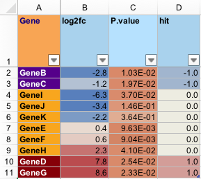
Value
Workbook object as defined by the openxlsx package
is returned invisibly with invisible(). This Workbook
can be used in argument wb to provide a speed boost when
saving multiple sheets to the same file.
See Also
Other jam export functions:
applyXlsxCategoricalFormat(),
applyXlsxConditionalFormat(),
readOpenxlsx(),
set_xlsx_colwidths(),
set_xlsx_rowheights()
Examples
# set up a test data.frame
set.seed(123);
lfc <- -3:3 + stats::rnorm(7)/3;
colorSub <- nameVector(
   rainbow2(7),
   LETTERS[1:7])
df <- data.frame(name=LETTERS[1:7],
   int=round(4^(1:7)),
   num=(1:7)*4-2 + stats::rnorm(7),
   fold=2^abs(lfc)*sign(lfc),
   lfc=lfc,
   pvalue=10^(-1:-7 + stats::rnorm(7)),
   hit=sample(c(-1,0,0,1,1), replace=TRUE, size=7));
df;
# write to tempfile for examples
if (check_pkg_installed("openxlsx")) {
   out_xlsx <- tempfile(pattern="writeOpenxlsx_", fileext=".xlsx")
   writeOpenxlsx(x=df,
      file=out_xlsx,
      sheetName="jamba_test",
      colorSub=colorSub,
      intColumns=2,
      numColumns=3,
      fcColumns=4,
      lfcColumns=5,
      pvalueColumns=6,
      hitColumn=7,
      freezePaneRow=2,
      freezePaneColumn=2,
      append=FALSE);
   # now read it back
   df_list <- readOpenxlsx(xlsx=out_xlsx);
   sdim(df_list)
}