| Type: | Package |
| Title: | Construct Flexible Urban Delineations |
| Version: | 0.2.2 |
| Description: | Enables the construction of flexible urban delineations that can be tailored to specific applications or research questions, see Van Migerode et al. (2024) <doi:10.1177/23998083241262545> and Van Migerode et al. (2025) <doi:10.5281/zenodo.15173220>. Originally developed to flexibly reconstruct the Degree of Urbanisation classification of cities, towns and rural areas developed by Dijkstra et al. (2021) <doi:10.1016/j.jue.2020.103312>. Now it also support a broader range of delineation approaches, using multiple datasets – including population, built-up area, and night-time light grids – and different thresholding methods. |
| License: | MIT + file LICENSE |
| URL: | https://github.com/cvmigero/flexurba, https://gitlab.kuleuven.be/spatial-networks-lab/research-projects/flexurba, https://flexurba-spatial-networks-lab-research-projects--e74426d1c66ecc.pages.gitlab.kuleuven.be |
| BugReports: | https://github.com/cvmigero/flexurba/issues |
| Depends: | R (≥ 3.5) |
| Imports: | data.table, dplyr, exactextractr, fastmatch, geos, ggplot2, ggspatial, grid, jsonlite, lifecycle, magrittr, nngeo, Rcpp, sf, terra (≥ 1.7-3), tidyterra, utils |
| Suggests: | knitr, rmarkdown, spelling, testthat (≥ 3.0.0) |
| LinkingTo: | Rcpp |
| VignetteBuilder: | knitr, rmarkdown |
| Config/Needs/website: | rmarkdown |
| Config/testthat/edition: | 3 |
| Encoding: | UTF-8 |
| Language: | en-GB |
| LazyData: | true |
| RoxygenNote: | 7.3.2 |
| NeedsCompilation: | yes |
| Packaged: | 2025-06-05 10:08:34 UTC; u0157090 |
| Author: | Céline Van Migerode
 [aut, cre],
Ate Poorthuis
[aut],
Ben Derudder
[aut],
KU Leuven [cph],
FWO [fnd] [aut, cre],
Ate Poorthuis
[aut],
Ben Derudder
[aut],
KU Leuven [cph],
FWO [fnd] |
| Maintainer: | Céline Van Migerode <celine.vanmigerode@kuleuven.be> |
| Repository: | CRAN |
| Date/Publication: | 2025-06-10 09:10:06 UTC |
Pipe operator
Description
See magrittr::[\%>\%][magrittr::pipe] for details.
Usage
lhs %>% rhs
Arguments
lhs |
A value or the magrittr placeholder. |
rhs |
A function call using the magrittr semantics. |
Value
The result of calling rhs(lhs).
Create the DEGURBA grid cell classification
Description
The function reconstructs the grid cell classification of the Degree of Urbanisation. The arguments of the function allow to adapt the standard specifications in the Degree of Urbanisation in order to construct an alternative version (see section "Custom specifications" below).
For more information about the Degree of Urbanisation methodology, see the methodological manual, GHSL Data Package 2022 and GHSL Data Package 2023.
Usage
DoU_classify_grid(
  data,
  level1 = TRUE,
  parameters = NULL,
  values = NULL,
  regions = FALSE,
  filename = NULL
)
Arguments
data |
path to the directory with the data, or named list with the data as returned by function |
level1 |
logical. Whether to classify the grid according to first hierarchical level ( |
parameters |
named list with the parameters to adapt the standard specifications in the Degree of Urbanisation classification. For more details, see section "Custom specifications" below. |
values |
vector with the values assigned to the different classes in the resulting classification:
|
regions |
logical. Whether to execute the classification in the memory-efficient pre-defined regions. For more details, see section "Regions" below (Note that this requires a large amount of memory). |
filename |
character. Output filename (with extension |
Value
SpatRaster with the grid cell classification
Classification rules
The Degree of Urbanisation consists of two hierarchical levels. In level 1, the cells of a 1 km² grid are classified in urban centres, urban clusters and rural cells (and water cells). In level 2, urban cluster are further divided in dense urban clusters, semi-dense urban clusters and suburbs or peri-urban cells. Rural cells are further divided in rural clusters, low density rural cells and very low density rural cells.
The detailed classification rules are as follows:
LEVEL 1:
-
Urban centres are identified as clusters of continuous grid cells (based on rook contiguity) with a minimum density of 1500 inhabitants per km² (or with a minimum built-up area; see section "Built-up area criterium" below), and a minimum total population of 50 000 inhabitants. Gaps smaller than 15 km² in the urban centres are filled and edges are smoothed by a 3x3-majority rule (see section "Edge smoothing" below).
-
Urban clusters are identified as clusters of continuous grid cells (based on queen contiguity) with a minimum density of 300 inhabitants per km², and a minimum total population of 5000 inhabitants.
-
Water cells contain no built-up area, no population, and less than 50% permanent land. All other cells not belonging to an urban centre or urban cluster are considered rural cells.
LEVEL 2:
-
Urban centres are identified as clusters of continuous grid cells (based on rook contiguity) with a minimum density of 1500 inhabitants per km² (or with a minimum built-up area; see section "Built-up area criterium" below), and a minimum total population of 50 000 inhabitants. Gaps smaller than 15 km² in the urban centres are filled and edges are smoothed by a 3x3-majority rule (see section "Edge smoothing" below).
-
Dense urban clusters are identified as clusters of continuous grid cells (based on rook contiguity) with a minimum density of 1500 inhabitants per km² (or with a minimum built-up area; see section "Built-up area criterium" below), and a minimum total population of 5000 inhabitants.
-
Semi-dense urban clusters are identified as clusters of continuous grid cells (based on rook contiguity) with a minimum density of 900 inhabitants per km², and a minimum total population of 2500 inhabitants, that are not within 2 km away from urban centres and dense urban clusters. Clusters that are within 2 km away are classified as suburban and peri-urban cells.
-
Rural clusters are clusters of continuous grid cells (based on queen contiguity) with a minimum density of 300 inhabitants per km², and a minimum total population of 500 inhabitants.
-
Low density rural cells are remaining cells with a population density less than 50 inhabitants per km².
-
Water cells contain no built-up area, no population, and less than 50% permanent land. All cells not belonging to an other class are considered very low density rural cells.
For more information about the Degree of Urbanisation methodology, see the methodological manual, GHSL Data Package 2022 and GHSL Data Package 2023.
Custom specifications
The function allows to change the standard specifications of the Degree of Urbanisation in order to construct an alternative version of the grid classification. Custom specifications can be passed in a named list by the argument parameters. The supported parameters with their default values are returned by the function DoU_get_grid_parameters() and are as follows:
LEVEL 1
-
UC_density_thresholdnumeric (default:1500).Minimum population density per permanent land of a cell required to belong to an urban centre
-
UC_size_thresholdnumeric (default:50000).Minimum total population size required for an urban centre
-
UC_contiguity_ruleinteger (default:4).Which cells are considered adjacent in urban centres:
4for rooks case (horizontal and vertical neighbours) or8for queens case (horizontal, vertical and diagonal neighbours) -
UC_built_criteriumlogical (default:TRUE).Whether to use the additional built-up area criterium (see section "Built-up area criterium" below). If
TRUE, not only cells that meet the population density requirement will be considered when delineating urban centres, but also cells with a built-up area per permanent land above theUC_built_threshold -
UC_built_thresholdnumeric or character (default:0.2).Additional built-up area threshold. Can be a value between
0and1, representing the minimum built-up area per permanent land, or"optimal"(see section "Built-up area criterium" below). Ignored whenUC_built_criteriumisFALSE. -
built_optimal_datacharacter / list (default:NULL).Path to the directory with the data, or named list with the data as returned by function
DoU_preprocess_grid()used to determine the optimal built threshold (see section "Built-up area criterium" below). Ignored whenUC_built_criteriumisFALSEor whenUC_built_thresholdis not"optimal". -
UC_smooth_poplogical (default:FALSE).Whether to smooth the population grid before delineating urban centres. If
TRUE, the population grid will be smoothed with a moving average of window sizeUC_smooth_pop_window. -
UC_smooth_pop_windowinteger (default:5).Size of the moving window used to smooth the population grid before delineating urban centres. Ignored when
UC_smooth_popisFALSE. -
UC_gap_filllogical (default:TRUE).Whether to perform gap filling. If
TRUE, gaps in urban centres smaller thanUC_max_gapare filled. -
UC_max_gapinteger (default:15).Gaps with an area smaller than this threshold in urban centres will be filled (unit is km²). Ignored when
UC_gap_fillisFALSE. -
UC_smooth_edgelogical (default:TRUE).Whether to perform edge smoothing. If
TRUE, edges of urban centres are smoothed with the functionUC_smooth_edge_fun. -
UC_smooth_edge_funcharacter / function (default:"majority_rule_R2023A").Function used to smooth the edges of urban centres. Ignored when
UC_smooth_edgeisFALSE. Possible values are:-
"majority_rule_R2022A"to use the edge smoothing algorithm in GHSL Data Package 2022 (see section "Edge smoothing" below) -
"majority_rule_R2023A"to use the edge smoothing algorithm in GHSL Data Package 2023 (see section "Edge smoothing" below) a custom function with a signature similar as
apply_majority_rule().
-
-
UCL_density_thresholdnumeric (default:300).Minimum population density per permanent land of a cell required to belong to an urban cluster
-
UCL_size_thresholdnumeric (default:5000).Minimum total population size required for an urban cluster
-
UCL_contiguity_ruleinteger (default:8).Which cells are considered adjacent in urban clusters:
4for rooks case (horizontal and vertical neighbours) or8for queens case (horizontal, vertical and diagonal neighbours) -
UCL_smooth_poplogical (default:FALSE).Whether to smooth the population grid before delineating urban clusters. If
TRUE, the population grid will be smoothed with a moving average of window sizeUCL_smooth_pop_window. -
UCL_smooth_pop_windowinteger (default:5).Size of the moving window used to smooth the population grid before delineating urban clusters. Ignored when
UCL_smooth_popisFALSE. -
water_land_thresholdnumeric (default:0.5).Maximum proportion of permanent land allowed in a water cell
-
water_pop_thresholdnumeric (default:0).Maximum population size allowed in a water cell
-
water_built_thresholdnumeric (default:0).Maximum built-up area allowed in a water cell
LEVEL 2
-
UC_density_thresholdnumeric (default:1500).Minimum population density per permanent land of a cell required to belong to an urban centre
-
UC_size_thresholdnumeric (default:50000).Minimum total population size required for an urban centre
-
UC_contiguity_ruleinteger (default:4).Which cells are considered adjacent in urban centres:
4for rooks case (horizontal and vertical neighbours) or8for queens case (horizontal, vertical and diagonal neighbours) -
UC_built_criteriumlogical (default:TRUE).Whether to use the additional built-up area criterium (see section "Built-up area criterium" below). If
TRUE, not only cells that meet the population density requirement will be considered when delineating urban centres, but also cells with a built-up area per permanent land above theUC_built_threshold -
UC_built_thresholdnumeric or character (default:0.2).Additional built-up area threshold. Can be a value between
0and1, representing the minimum built-up area per permanent land, or"optimal"(see section "Built-up area criterium" below). Ignored whenUC_built_criteriumisFALSE. -
built_optimal_datacharacter / list (default:NULL).Path to the directory with the data, or named list with the data as returned by function
DoU_preprocess_grid()used to determine the optimal built threshold (see section "Built-up area criterium" below). Ignored whenUC_built_criteriumisFALSEor whenUC_built_thresholdis not"optimal". -
UC_smooth_poplogical (default:FALSE).Whether to smooth the population grid before delineating urban centres. If
TRUE, the population grid will be smoothed with a moving average of window sizeUC_smooth_pop_window. -
UC_smooth_pop_windowinteger (default:5).Size of the moving window used to smooth the population grid before delineating urban centres. Ignored when
UC_smooth_popisFALSE. -
UC_gap_filllogical (default:TRUE).Whether to perform gap filling. If
TRUE, gaps in urban centres smaller thanUC_max_gapare filled. -
UC_max_gapinteger (default:15).Gaps with an area smaller than this threshold in urban centres will be filled (unit is km²). Ignored when
UC_gap_fillisFALSE. -
UC_smooth_edgelogical (default:TRUE).Whether to perform edge smoothing. If
TRUE, edges of urban centres are smoothed with the functionUC_smooth_edge_fun. -
UC_smooth_edge_funcharacter / function (default:"majority_rule_R2023A").Function used to smooth the edges of urban centres. Ignored when
UC_smooth_edgeisFALSE. Possible values are:-
"majority_rule_R2022A"to use the edge smoothing algorithm in GHSL Data Package 2022 (see section "Edge smoothing" below) -
"majority_rule_R2023A"to use the edge smoothing algorithm in GHSL Data Package 2023 (see section "Edge smoothing" below) a custom function with a signature similar as
apply_majority_rule().
-
-
DUC_density_thresholdnumeric (default:1500).Minimum population density required for a dense urban cluster
-
DUC_size_thresholdnumeric (default:5000).Minimum total population size required for a dense urban cluster
-
DUC_built_criteriumlogical (default:TRUE).Whether to use the additional built-up area criterium (see section "Built-up area criterium" below). If
TRUE, not only cells that meet the population density requirement will be considered when delineating dense urban clusters, but also cells with a built-up area per permanent land above theDUC_built_threshold -
DUC_built_thresholdnumeric or character (default:0.2).Additional built-up area threshold. Can be a value between
0and1, representing the minimum built-up area per permanent land, or"optimal"(see section "Built-up area criterium" below). Ignored whenDUC_built_criteriumisFALSE. -
DUC_contiguity_ruleinteger (default:4).Which cells are considered adjacent in dense urban clusters:
4for rooks case (horizontal and vertical neighbours) or8for queens case (horizontal, vertical and diagonal neighbours) -
SDUC_density_thresholdnumeric (default:900).Minimum population density per permanent land of a cell required to belong to a semi-dense urban cluster
-
SDUC_size_thresholdnumeric (default:2500).Minimum total population size required for a semi-dense urban cluster
-
SDUC_contiguity_ruleinteger (default:4).Which cells are considered adjacent in semi-dense urban clusters:
4for rooks case (horizontal and vertical neighbours) or8for queens case (horizontal, vertical and diagonal neighbours) -
SDUC_buffer_sizeinteger (default:2).The distance to urban centres and dense urban clusters required for a semi-dense urban cluster
-
SUrb_density_thresholdnumeric (default:300).Minimum population density per permanent land of a cell required to belong to a suburban or peri-urban area
-
SUrb_size_thresholdnumeric (default:5000).Minimum total population size required for a suburban or peri-urban area
-
SUrb_contiguity_ruleinteger (default:8).Which cells are considered adjacent in suburban or peri-urban area:
4for rooks case (horizontal and vertical neighbours) or8for queens case (horizontal, vertical and diagonal neighbours) -
RC_density_thresholdnumeric (default:300).Minimum population density per permanent land of a cell required to belong to a rural cluster
-
RC_size_thresholdnumeric (default:500).Minimum total population size required for a rural cluster
-
RC_contiguity_ruleinteger (default:8).Which cells are considered adjacent in rural clusters:
4for rooks case (horizontal and vertical neighbours) or8for queens case (horizontal, vertical and diagonal neighbours) -
LDR_density_thresholdnumeric (default:50).Minimum population density per permanent land of a low density rural grid cell
-
water_land_thresholdnumeric (default:0.5).Maximum proportion of permanent land allowed in a water cell
-
water_pop_thresholdnumeric (default:0).Maximum population size allowed in a water cell
-
water_built_thresholdnumeric (default:0).Maximum built-up area allowed in a water cell
Built-up area criterium
In Data Package 2022, the Degree of Urbanisation includes an optional built-up area criterium to account for the presence of office parks, shopping malls, factories and transport infrastructure. When the setting is enabled, urban centres (and dense urban clusters) are created using both cells with a population density of at least 1500 inhabitants per km² and cells that have at least 50% built-up area on permanent land. For more information: see GHSL Data Package 2022, footnote 25. The parameter settings UC_built_criterium=TRUE and UC_built_threshold=0.5 (level 1 & 2) and DUC_built_criterium=TRUE and DUC_built_threshold=0.5 (level 2) reproduce this built-up area criterium in urban centres and dense urban clusters respectively.
In Data Package 2023, the built-up area criterium is slightly adapted and renamed to the "Reduce Fragmentation Option". Instead of using a fixed threshold of built-up area per permanent land of 50%, an "optimal" threshold is employed. The optimal threshold is dynamically identified as the global average built-up area proportion in clusters with a density of at least 1500 inhabitants per permanent land with a minimum population of 5000 people. We determined empirically that this optimal threshold is 20% for the data of 2020. For more information: see GHSL Data Package 2023, footnote 30. The "Reduce Fragmentation Option" can be reproduced with the parameter settings UC_built_criterium=TRUE and UC_built_threshold="optimal" (level 1 & 2) and DUC_built_criterium=TRUE and DUC_built_threshold="optimal" (level 2). In addition, the parameter built_optimal_data must contain the path to the directory with the (global) data to compute the optimal built-up area threshold.
Edge smoothing
In Data Package 2022, edges of urban centres are smoothed by an iterative majority rule. The majority rule works as follows: if a cell has at least five of the eight surrounding cells belonging to an unique urban centre, then the cell is added to that urban centre. The process is iteratively repeated until no more cells are added. The parameter setting UC_smooth_edge=TRUE and UC_smooth_edge_fun="majority_rule_R2022A" reproduces this edge smoothing rule.
In Data Package 2023, the majority rule is slightly adapted. A cell is added to an urban centre if the majority of the surrounding cells belongs to an unique urban centre, with majority only computed among populated or land cells (proportion of permanent land > 0.5). In addition, cells with permanent water are never added to urban centres. The process is iteratively repeated until no more cells are added. For more information: see GHSL Data Package 2023, footnote 29. The parameter setting UC_smooth_edge=TRUE and UC_smooth_edge_fun="majority_rule_R2023A" reproduces this edge smoothing rule.
Regions
Because of the large amount of data at a global scale, the grid classification procedure is quite memory-consuming. To optimise the procedure, we divided the world in 9 pre-defined regions. These regions are the smallest grouping of GHSL tiles while ensuring that no continuous land mass is split into two different regions (for more information, see the figure below and GHSL_tiles_per_region).
If regions=TRUE, a global grid classification is created by (1) executing the grid classification procedure separately in the 9 pre-defined regions, and (2) afterwards merging these classifications together. The argument data should contain the path to a directory with the data of all pre-defined regions (for example as created by download_GHSLdata(... extent="regions"). Note that although the grid classification is optimised, it still takes approx. 145 minutes and requires 116 GB RAM to execute the grid classification with the standard parameters (performed on a Kubernetes server with 32 cores and 256 GB RAM). For a concrete example on how to construct the grid classification on a global scale, see vignette("vig3-DoU-global-scale").
Examples
# load the data
data_belgium <- DoU_load_grid_data_belgium()

# classify with standard parameters:
classification1 <- DoU_classify_grid(data = data_belgium)


# classify with custom parameters:
classification2 <- DoU_classify_grid(
  data = data_belgium,
  parameters = list(
    UC_density_threshold = 3000,
    UC_size_threshold = 75000,
    UC_gap_fill = FALSE,
    UC_smooth_edge = FALSE,
    UCL_contiguity_rule = 4
  )
)
Create the DEGURBA grid cell classification of rural cells
Description
The Degree of Urbanisation identifies rural cells as all cells not belonging to an urban centre or urban cluster.
For more information about the Degree of Urbanisation methodology, see the methodological manual, GHSL Data Package 2022 and GHSL Data Package 2023.
Usage
DoU_classify_grid_rural(data, classification, value = 1)
Arguments
data |
path to the directory with the data, or named list with the data as returned by function |
classification |
SpatRaster. A grid with the classification of urban centres and urban clusters to which the classification of rural cells will be added. Note that the grid will be adapted in-place. |
value |
integer. Value assigned to rural cells in the resulting grid |
Value
SpatRaster with the grid cell classification of rural cells
Examples
data_belgium <- DoU_load_grid_data_belgium()
classification <- DoU_classify_grid_urban_centres(data_belgium)
classification <- DoU_classify_grid_urban_clusters(data_belgium, classification = classification)
classification <- DoU_classify_grid_rural(data_belgium, classification = classification)
DoU_plot_grid(classification)
Create the DEGURBA grid cell classification of urban centres
Description
The Degree of Urbanisation identifies urban centres as clusters of continuous grid cells (based on rook contiguity) with a minimum density of 1500 inhabitants per km² (or with a minimum built-up area; see details), and a minimum total population of 50 000 inhabitants. Gaps smaller than 15 km² in the urban centres are filled and edges are smoothed by a 3x3-majority rule (see details).
For more information about the Degree of Urbanisation methodology, see the methodological manual, GHSL Data Package 2022 and GHSL Data Package 2023.
The arguments of the function allow to adapt the standard specifications in the Degree of Urbanisation in order to construct an alternative version of the grid classification.
Usage
DoU_classify_grid_urban_centres(
  data,
  density_threshold = 1500,
  size_threshold = 50000,
  contiguity_rule = 4,
  built_criterium = TRUE,
  built_threshold = 0.2,
  smooth_pop = FALSE,
  smooth_pop_window = 5,
  gap_fill = TRUE,
  max_gap = 15,
  smooth_edge = TRUE,
  smooth_edge_fun = "majority_rule_R2023A",
  value = 3
)
Arguments
data |
path to the directory with the data, or named list with the data as returned by function |
density_threshold |
numeric. Minimum population density per permanent land of a cell required to belong to an urban centre |
size_threshold |
numeric. Minimum total population size required for an urban centre |
contiguity_rule |
integer. Which cells are considered adjacent: |
built_criterium |
logical. Whether to use the additional built-up area criterium (see details). If |
built_threshold |
numeric. Additional built-up area threshold. A value between |
smooth_pop |
logical. Whether to smooth the population grid before delineating urban centres. If |
smooth_pop_window |
integer. Size of the moving window used to smooth the population grid before delineating urban centres. Ignored when |
gap_fill |
logical. Whether to perform gap filling. If |
max_gap |
integer. Gaps with an area smaller than this threshold in urban centres will be filled (unit is km²). Ignored when |
smooth_edge |
logical. Whether to perform edge smoothing. If |
smooth_edge_fun |
character / function. Function used to smooth the edges of urban centres. Ignored when
|
value |
integer. Value assigned to urban centres in the resulting grid |
Details
-
Optional built-up area criterium
In Data Package 2022, the Degree of Urbanisation includes an optional built-up area criterium to account for the presence of office parks, shopping malls, factories and transport infrastructure. When the setting is enabled, urban centres are created using both cells with a population density of at least 1500 inhabitants per km² and cells that have at least 50% built-up area on permanent land. For more information: see GHSL Data Package 2022, footnote 25. The parameter setting built_criterium=TRUE and built_threshold=0.5 reproduces this built-up area criterium.
In Data Package 2023, the built-up area criterium is slightly adapted and renamed to the "Reduce Fragmentation Option". Instead of using a fixed threshold of built-up area per permanent land of 50%, an "optimal" threshold is employed. The optimal threshold is dynamically identified as the global average built-up area proportion in clusters with a density of at least 1500 inhabitants per permanent land with a minimum population of 5000 people. For more information: see GHSL Data Package 2023, footnote 30. The optimal built-up threshold can be computed with the function DoU_get_optimal_builtup(). We determined empirically that this optimal threshold is 20% for the data of 2020.
-
Edge smoothing: majority rule algorithm
In Data Package 2022, edges of urban centres are smoothed by an iterative majority rule. The majority rule works as follows: if a cell has at least five of the eight surrounding cells belonging to an unique urban centre, then the cell is added to that urban centre. The process is iteratively repeated until no more cells are added. The parameter setting smooth_edge=TRUE and smooth_edge_fun="majority_rule_R2022A" reproduces this edge smoothing rule.
In Data Package 2023, the majority rule is slightly adapted. A cell is added to an urban centre if the majority of the surrounding cells belongs to an unique urban centre, with majority only computed among populated or land cells (proportion of permanent land > 0.5). In addition, cells with permanent water are never added to urban centres. The process is iteratively repeated until no more cells are added. For more information: see GHSL Data Package 2023, footnote 29. The parameter setting smooth_edge=TRUE and smooth_edge_fun="majority_rule_R2023A" reproduces this edge smoothing rule.
Value
SpatRaster with the grid cell classification of urban centres
Examples
data_belgium <- DoU_load_grid_data_belgium()

# standard parameters of the Degree of Urbanisation:
classification1 <- DoU_classify_grid_urban_centres(data_belgium)
DoU_plot_grid(classification1)

# with custom parameters:
classification2 <- DoU_classify_grid_urban_centres(data_belgium,
  density_threshold = 1000,
  gap_fill = FALSE,
  smooth_edge = FALSE
)
DoU_plot_grid(classification2)
Create the DEGURBA grid cell classification of urban clusters
Description
The Degree of Urbanisation identifies urban clusters as clusters of continuous grid cells (based on queen contiguity) with a minimum density of 300 inhabitants per km², and a minimum total population of 5000 inhabitants.
For more information about the Degree of Urbanisation methodology, see the methodological manual, GHSL Data Package 2022 and GHSL Data Package 2023.
The arguments of the function allow to adapt the standard specifications in the Degree of Urbanisation in order to construct an alternative version of the grid classification.
Usage
DoU_classify_grid_urban_clusters(
  data,
  classification,
  density_threshold = 300,
  size_threshold = 5000,
  contiguity_rule = 8,
  smooth_pop = FALSE,
  smooth_pop_window = 5,
  value = 2
)
Arguments
data |
path to the directory with the data, or named list with the data as returned by function |
classification |
SpatRaster. A grid with the classification of urban centres to which the classification of urban clusters will be added. Note that the grid will be adapted in-place. |
density_threshold |
numeric. Minimum population density per permanent land of a cell required to belong to an urban cluster |
size_threshold |
numeric. Minimum total population size required for an urban cluster |
contiguity_rule |
integer. Which cells are considered adjacent: |
smooth_pop |
logical. Whether to smooth the population grid before delineating urban clusters. If |
smooth_pop_window |
integer. Size of the moving window used to smooth the population grid before delineating urban clusters. Ignored when |
value |
integer. Value assigned to urban clusters in the resulting grid |
Value
SpatRaster with the grid cell classification of urban clusters
Examples
data_belgium <- DoU_load_grid_data_belgium()
classification <- DoU_classify_grid_urban_centres(data_belgium)
classification <- DoU_classify_grid_urban_clusters(data_belgium, classification = classification)
DoU_plot_grid(classification)
Create the DEGURBA grid cell classification of water cells
Description
The Degree of Urbanisation identifies water cells as cells with no built-up area, no population, and less than 50% permanent land.
For more information about the Degree of Urbanisation methodology, see the methodological manual, GHSL Data Package 2022 and GHSL Data Package 2023.
The arguments of the function allow to adapt the standard specifications in the Degree of Urbanisation in order to construct an alternative version of the grid classification.
Usage
DoU_classify_grid_water(
  data,
  classification = NULL,
  water_land_threshold = 0.5,
  water_pop_threshold = 0,
  water_built_threshold = 0,
  value = 0,
  allow_overwrite = c(1)
)
Arguments
data |
path to the directory with the data, or named list with the data as returned by function |
classification |
SpatRaster. A grid to which the classification of water cells will be added. The grid can already contain the classification or urban centres, urban clusters and rural grid cell, but this is not mandatory. Note that the grid will be adapted in-place. |
water_land_threshold |
numeric. Maximum proportion of permanent land allowed in a water cell |
water_pop_threshold |
numeric. Maximum population size allowed in a water cell |
water_built_threshold |
numeric. Maximum built-up area allowed in a water cell |
value |
integer. Value assigned to water cells in the resulting grid |
allow_overwrite |
vector. Values in |
Value
SpatRaster with the grid cell classification of water cells
Examples
data_belgium <- DoU_load_grid_data_belgium()
classification <- DoU_classify_grid_urban_centres(data_belgium)
classification <- DoU_classify_grid_urban_clusters(data_belgium, classification = classification)
classification <- DoU_classify_grid_rural(data_belgium, classification = classification)
classification <- DoU_classify_grid_water(data_belgium, classification = classification)
DoU_plot_grid(classification)
Create the DEGURBA spatial units classification
Description
The function reconstructs the spatial units classification of the Degree of Urbanisation based on the grid cell classification.
Usage
DoU_classify_units(
  data,
  id = "UID",
  level1 = TRUE,
  values = NULL,
  official_workflow = TRUE,
  rules_from_2021 = FALSE,
  filename = NULL
)
Arguments
data |
named list with the required data, as returned by the function |
id |
character. Unique column in the |
level1 |
logical. Whether to classify the spatial units according to first hierarchical level ( |
values |
vector with the values assigned to the different classes in the resulting units classification:
|
official_workflow |
logical. Whether to employ the official workflow of the GHSL ( |
rules_from_2021 |
logical. Whether to employ the original classification rules as described in the 2021 version of the DEGURBA manual. The DEUGURBA Level 2 unit classification rules have been modified in July 2024. By default, the function uses the most recent rules as described in the online version of the methodological manual. For more details, see section "Modification of the unit classification rules" below. |
filename |
character. Output filename (csv). The resulting classification together with a metadata file (in JSON format) will be saved if |
Value
dataframe with for each spatial unit the classification and the share of population per grid class
Classification rules
The Degree of Urbanisation consists of two hierarchical levels. In level 1, the spatial units are classified in cities, towns and semi-dense areas, and rural areas. In level 2, towns and semi-dense areas are further divided in dense towns, semi-dense towns and suburban or peri-urban areas. Rural areas are further divided in villages, dispersed rural areas and mostly uninhabited areas.
The detailed classification rules are as follows:
LEVEL 1:
-
Cities: units that have at least 50% of their population in urban centres
-
Towns and semi-dense areas: units that have less than 50% of their population in urban centres and no more than 50% of their population in rural grid cells
-
Rural areas: units that have more then 50% of their population in rural grid cells
LEVEL 2:
-
Cities: units that have at least 50% of their population in urban centres
-
Dense towns: units that have at least 50% of their population in the combination of urban centres and dense urban clusters
-
Semi-dense towns: units that have less than 50% of their population in the combination of urban centres and dense urban clusters, or have less than 50% of their population in the combination of suburban and peri-urban cells and rural grid cells
-
Suburbs or peri-urban areas: units that have at least 50% of their population in the combination of suburban and peri-urban cells and rural grid cells
-
Villages: units that have at least 50% of their population in the combination of urban centres, urban clusters and rural clusters
-
Dispersed rural areas: units that have less than 50% of their population in the combination of urban centres, urban clusters and rural clusters, or have less than 50% of their population in very low-density rural grid cells
-
Mostly uninhabited areas: units that have at least 50% of their population in very low-density rural grid cells
Workflow
The classification of small spatial units requires a vector layer with the small spatial units, a raster layer with the grid cell classification, and a raster layer with the population grid. Standard, a population grid of 100 m resolution is used by the Degree of Urbanisation.
The function includes two different workflows to establish the spatial units classification based on these three data sources.
Official workflow according to the GHSL:
For the official workflow, the three layers should be pre-processed by DoU_preprocess_units(). In this function, the classification grid and population grid are resampled to a user-defined resample_resolution with the nearest neighbour algorithm (the Degree of Urbanisation uses standard a resample resolution of 50 m). In doing this, the values of the population grid are divided by the oversampling ratio (for example: going from a resolution of 100 m to a resolution of 50 m, the values of the grid are divided by 4).
Afterwards, the spatial units classification is constructed with DoU_classify_units() as follows. The vector layer with small spatial units is rasterised to match the population and classification grid. Based on the overlap of the three grids, the share of population per flexurba grid class is computed per spatial unit with a zonal statistics procedure. The units are subsequently classified according to the classification rules (see above).
Apart from this, there are two special cases. First, if a unit has no population, it is classified according to the share of land area in each of the flexurba grid classes (computed with a zonal statistics procedure). Second, if a unit initially could not be rasterised (can occur if the area of the unit < resample_resolution), then it is processed separately as follows. The unit is individually rasterised by all touching cells. The unit is classified according to the share of population in the flexurba grid classes in these touching cells. However, to avoid double counting of population, no population is assigned to the unit in the result.
For more information about the official workflow to construct the units classification, see GHSL Data Package 2023 (Section 2.7.2.3).
Alternative workflow:
Besides the official workflow of the GHSL, the function also includes an alternative workflow to construct the spatial units classification. The alternative workflow does not require rasterising the spatial units layer, but relies on the overlap between the spatial units layer and the grid layers.
The three layers should again be pre-processed by the function DoU_preprocess_units(), but this time without resampling_resolution. For the classification in DoU_classify_units(), the function exactextractr::exact_extract() is used to (1) overlay the grids with the spatial units layer, and (2) summarise the values of the population grid and classification grid per unit. The units are subsequently classified according to the classification rules (see above). As an exception, if a unit has no population, it is classified according to the share of land area in each of the flexurba grid classes. The alternative workflow is slightly more efficient as it does not require resampling the population and classification grids and rasterising the spatial units layer.
Modification of the unit classification rules
The unit classification rules of Level 2 of DEGURBA were updated in July 2024. By default, the function DoU_classify_units() applies the latest classification rules, as described in the online version of the methodological manual. However, you can also use the original 2021 classification rules if desired, by setting the argument rules_from_2021 to TRUE. In that case, the rules to classify units are as follows:
-
Cities: units that have at least 50% of their population in urban centres
-
Dense towns: units that have a larger share of the population in dense urban clusters than in semi-dense urban clusters, and that have a larger share of the population in dense + semi-dense urban clusters than in suburban or peri-urban cells
-
Semi-dense towns: units that have a larger share of the population in semi-dense urban clusters than in semi-dense urban clusters, and that have a larger share of the population in dense + semi-dense urban clusters than in suburban or peri-urban cells
-
Suburbs or peri-urban areas: units that have a larger share in suburban or peri-urban cells than in dense + semi-dense urban clusters
-
Villages: units that have the largest share of their rural grid cell population living in rural clusters
-
Dispersed rural areas: units that have the largest share of their rural grid cell population living in low density rural grid cells
-
Mostly uninhabited areas: units that have the largest share of their rural grid cell population living in very low density rural grid cells
Examples
# load the grid data
data_belgium <- flexurba::DoU_load_grid_data_belgium()
# load the units and filter for West-Flanders
units_data <- flexurba::units_belgium %>%
  dplyr::filter(GID_2 == "30000")
# classify the grid
classification <- DoU_classify_grid(data = data_belgium)


# official workflow
data1 <- DoU_preprocess_units(
  units = units_data,
  classification = classification,
  pop = data_belgium$pop,
  resample_resolution = 50
)
units_classification1 <- DoU_classify_units(data1)


# alternative workflow
data2 <- DoU_preprocess_units(
  units = units_data,
  classification = classification,
  pop = data_belgium$pop
)
units_classification2 <- DoU_classify_units(data2, official_workflow = FALSE)

# spatial units classification, dissolved at level 3 (Belgian districts)
data3 <- DoU_preprocess_units(
  units = units_data,
  classification = classification,
  pop = data_belgium$pop,
  dissolve_units_by = "GID_3"
)
units_classification3 <- DoU_classify_units(data3, id = "GID_3")
Get the parameters for the DEGURBA grid cell classification
Description
The argument parameter of the function DoU_classify_grid() allows to adapt the standard specifications in the Degree of Urbanisation in order to construct an alternative version of the grid classification. This function returns a named list with the standard parameters.
Usage
DoU_get_grid_parameters(level1 = TRUE)
Arguments
level1 |
logical. Whether to return the standard parameters of level 1 of the Degree of Urbanisation ( |
Value
named list with the standard parameters
Examples
# example on how to employ the function to construct
# an alternative version of the grid classification:
# get the standard parameters
parameters <- DoU_get_grid_parameters()

# adapt the standard parameters
parameters$UCL_density_threshold <- 500
parameters$UCL_size_threshold <- 6000
parameters$UCL_smooth_pop <- TRUE
parameters$UCL_smooth_pop_window <- 7

# load the data
grid_data <- DoU_load_grid_data_belgium()

# use the adapted parameters to construct a grid cell classification
classification <- DoU_classify_grid(
  data = grid_data,
  parameters = parameters
)
Get the optimal built-up area threshold
Description
In Data Package 2023, the Degree of Urbanisation includes a "Reduce Fragmentation Option" to account for the presence of office parks, shopping malls, factories and transport infrastructure. When the setting is enabled, urban centres are created using both cells with a population density of at least 1500 inhabitants per km² and cells that have an "optimal" built-up area on permanent land. This function can be used to determine this "optimal" threshold value.
The optimal threshold is dynamically identified as the global average built-up area proportion in clusters with a density of at least 1500 inhabitants per permanent land with a minimum population of 5000 people. We empirically discovered that the Degree of Urbanisation uses the rounded up (ceiled) optimal threshold to two decimal places.
For more information: see GHSL Data Package 2023, footnote 30. The arguments of the function allow to adapt the standard specifications in order to determine an alternative "optimal" threshold.
Usage
DoU_get_optimal_builtup(
  data,
  density_threshold = 1500,
  size_threshold = 5000,
  directions = 4
)
Arguments
data |
path to the directory with the data, or named list with the data as returned by function |
density_threshold |
numeric. Minimum population density per permanent land |
size_threshold |
numeric. Minimum population size |
directions |
integer. Which cells are considered adjacent: |
Value
optimal built-up area threshold
Examples
data_belgium <- DoU_load_grid_data_belgium()

# determine the optimal built-up threshold with standard specifications
DoU_get_optimal_builtup(data_belgium)

# determine the optimal built-up threshold with custom specification
DoU_get_optimal_builtup(data_belgium,
  density_threshold = 1000,
  size_threshold = 3500,
  directions = 8
)
Load the grid data for Belgium to reconstruct DEGURBA classification
Description
The function loads the data required to execute the grid classification of the Degree of Urbanisation for Belgium with the function DoU_preprocess_grid().
The data was constructed with the code below:
# download the GHSL data on a global scale
download_GHSLdata(output_directory = "inst/extdata/global")

# crop the global grid to Belgium
crop_GHSLdata(extent = terra::ext(192000, 485000, 5821000, 6030000),
              global_directory = "inst/extdata/global",
              output_directory = "inst/extdata/belgium")
Usage
DoU_load_grid_data_belgium()
Value
named list with the data of Belgium required for the grid classification of the Degree of Urbanisation.
Examples
DoU_load_grid_data_belgium()
Plot the grid cell classification
Description
The function can be used to plot the results of the grid cell classification of the Degree of Urbanisation. The implementation relies upon the function tidyterra::geom_spatraster(). By default, the standard color scheme of the Global Human Settlement Layer (GHSL) is used (see GHSL Data Package 2023), but this can be altered by the palette argument.
Note that the function is computational quite heavy for large spatial extents (regional or global scale). It is advised to use the extent argument to plot only a selection of the grid classification.
Usage
DoU_plot_grid(
  classification,
  extent = NULL,
  level1 = TRUE,
  palette = NULL,
  labels = NULL,
  title = NULL,
  scalebar = FALSE,
  filename = NULL
)
Arguments
classification |
SpatRaster / character. A SpatRaster with the grid cell classification or the path to the grid cell classification file |
extent |
SpatExtent. If not |
level1 |
logical. Whether the grid is classified according to level 1 of the Degree of Urbanisation ( |
palette |
named vector with the color palette used to plot the grid cell classification. If |
labels |
vector with the labels used in the legend. If |
title |
character. Title of the plot.t |
scalebar |
logical. Whether to add a scale bar to the plot. |
filename |
character. Path to the location to save the plot |
Value
ggplot object
Examples
classification <- DoU_classify_grid(DoU_load_grid_data_belgium())

# plot with standard color scheme
DoU_plot_grid(classification)

# use custom palette and labels
DoU_plot_grid(classification,
  palette = c("3" = "#e16c72", "2" = "#fac66c", "1" = "#97c197", "0" = "#acd3df"),
  labels = c("UC", "UCL", "RUR", "WAT")
)
Plot the spatial units classification
Description
The function can be used to plot the results of the spatial units classification of the Degree of Urbanisation. The implementation relies upon the function ggplot2::geom_sf(). By default, the standard color scheme of the Global Human Settlement Layer (GHSL) is used (see GHSL Data Package 2023), but this can be altered by the palette argument.
Note that the function is computational quite heavy for large spatial extents (regional or global scale). It is advised to use the extent argument to plot only a selection of the spatial units classification.
Usage
DoU_plot_units(
  units,
  classification = NULL,
  level1 = TRUE,
  extent = NULL,
  column = NULL,
  palette = NULL,
  labels = NULL,
  title = NULL,
  scalebar = FALSE,
  filename = NULL
)
Arguments
units |
object of class |
classification |
dataframe with the classification of the spatial units, as returned by |
level1 |
logical. Whether the spatial units are classified according to level 1 of the Degree of Urbanisation ( |
extent |
SpatExtent or an object of class "bbox" ( |
column |
character. Column name of the spatial units classification. By default, |
palette |
named vector with the color palette used to plot the spatial units classification. If |
labels |
vector with the labels used in the legend. If |
title |
character. Title of the plot. |
scalebar |
logical. Whether to add a scale bar to the plot. |
filename |
character. Path to the location to save the plot |
Value
ggplot object
Examples
# get spatial units classification
data_belgium <- DoU_load_grid_data_belgium()
grid_classification <- DoU_classify_grid(data_belgium)
data1 <- DoU_preprocess_units(
  units = flexurba::units_belgium,
  classification = grid_classification,
  pop = data_belgium$pop
)
units_classification <- DoU_classify_units(data1)

# plot using the standard color palette
DoU_plot_units(data1$units, units_classification)

# plot using custom palette and labels
DoU_plot_units(data1$units, units_classification,
  palette = c("3" = "#e16c72", "2" = "#fac66c", "1" = "#97c197"),
  labels = c("C", "T", "R")
)
Preprocess the data for the DEGURBA grid cell classification
Description
The grid cell classification of the Degree of Urbanisation requires three different inputs:
a built-up area grid
a population grid
a land grid
The function rescales the built-up area and land grid if necessary (see details) and computes the population and built-up area per permanent land by dividing the respective grids by the land layer.
Usage
DoU_preprocess_grid(
  directory,
  filenames = c("BUILT_S.tif", "POP.tif", "LAND.tif"),
  rescale_land = TRUE,
  rescale_built = TRUE
)
Arguments
directory |
character. Path to the directory where the three input grids are saved (for example generated by the function |
filenames |
vector of length 3 with the filenames of the built-up area, population and land grid |
rescale_land |
logical. Whether to rescale the values of the land grid (see details) |
rescale_built |
logical. Whether to rescale the values of the built-up area grid (see details) |
Details
The values of the land grid and built-up area grid should range from 0 to 1, representing the proportion of permanent land and built-up area respectively. However, the grid values of the GHSL are standard in m². With a cell size of 1 km², the values thus range from 0 to 1 000 000. The two grids can be rescaled by setting rescale_land=TRUE and/or rescale_built=TRUE respectively.
Value
named listed with the required data to execute the grid cell classification procedure. The list contains following elements:
-
built: built-up area grid -
pop: population grid -
land: land grid -
pop_per_land: population per area of permanent land -
built_per_land: built-up area per permanent land -
metadata_BUILT_S: the metadata of the built-up area grid -
metadata_POP: the metadata of the population grid -
metadata_LAND: the metadata of the land grid.
Preprocess the data for the DEGURBA spatial units classification
Description
The spatial units classification of the Degree of Urbanisation requires three different inputs (all input sources should be in the Mollweide coordinate system):
a vector layer with the small spatial units
a raster layer with the grid cell classification of the Degree of Urbanisation
a raster layer with the population grid
The three input layers are pre-processed as follows. The classification grid and population grid are resampled to the resample_resolution with the nearest neighbour algorithm. In doing this, the values of the population grid are divided by the oversampling ratio (for example: going from a resolution of 100 m to a resolution of 50 m, the values of the grid are divided by 4).
In addition, the function makes sure the extents of the three input layers match. If the bounding box of the units layer is smaller than the extent of the grids, then the grids are cropped to the bounding box of the units layer. Alternatively, if the units layer covers a larger area than the grids, then the units that do not intersect with the grids are discarded (and a warning message is printed). This ensures that the classification algorithm runs efficiently and does not generate any incorrect classifications due to missing data.
More information about the pre-processing workflow, see GHSL Data Package 2023 (Section 2.7.2.3).
Usage
DoU_preprocess_units(
  units,
  classification,
  pop,
  resample_resolution = NULL,
  dissolve_units_by = NULL
)
Arguments
units |
character / object of class |
classification |
character / SpatRaster. Path to the grid cell classification of the Degree of Urbanisation, or SpatRaster with the grid cell classification |
pop |
character / SpatRaster. Path to the population grid, or SpatRaster with the population grid |
resample_resolution |
numeric. Resolution to which the grids are resampled during pre-processing. If |
dissolve_units_by |
character. If not |
Value
named list with the required data to execute the spatial units classification procedure, and their metadata. The list contains the following elements:
-
classification: the (resampled and cropped) grid cell classification layer -
pop: the (resampled and cropped) population grid -
units: the (dissolved and filtered) spatial units (object of classsf) -
metadata: named list with the metadata of the input files. It contains the elementsunits,classificationandpop(with paths to the respective data sources),resample_resolutionanddissolve_units_byif notNULL. (Note that when the input sources are passed by object , the metadata might be empty).
Examples
# load the grid data
grid_data <- flexurba::DoU_load_grid_data_belgium()
# load the units and filter for West-Flanders
units_data <- flexurba::units_belgium %>%
  dplyr::filter(GID_2 == "30000")
# classify the grid
classification <- DoU_classify_grid(data = grid_data)

# preprocess the data for units classification
data1 <- DoU_preprocess_units(
  units = units_data,
  classification = classification,
  pop = grid_data$pop,
  resample_resolution = 50
)

# preprocess the data for units classification at level 3 (Belgian districts)
data2 <- DoU_preprocess_units(
  units = units_data,
  classification = classification,
  pop = grid_data$pop,
  resample_resolution = 50,
  dissolve_units_by = "GID_3"
)
A dataframe with existing GHSL tiles
Description
The Global Human Settlement Layer (GHSL) divides the world into different rectangular areas called "tiles". These tiles can be used to download the GHSL products from the website (see GHSL Download page).
The dataset GHSL_tiles contains the geometry and metadata of all valid tiles.
Usage
GHSL_tiles
Format
GHSL_tiles
A dataframe with 375 rows and 6 columns
- tile_id
id of the tile
- left, top, right, bottom
The coordinates of the bounding box of the tile (in Mollweide, EPSG: 54009)
- geometry
sfc_POLYGONgeometry of the tile
Details
Spatial distribution of the GHSL tiles:
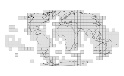
Source
https://ghsl.jrc.ec.europa.eu/download/GHSL_data_54009_shapefile.zip
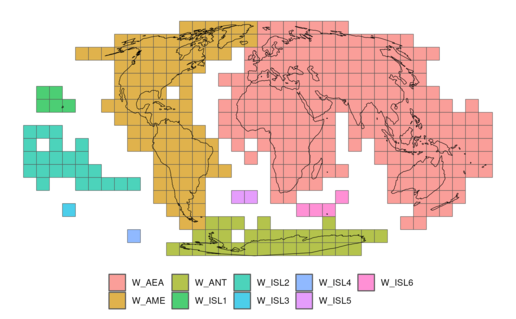
Division of GHSL tiles in 9 regions
Description
The Global Human Settlement Layer (GHSL) divides the world into different rectangular tiles. To execute the Degree of Urbanisation in a memory-efficient manner, we grouped these tiles into 9 different regions. These regions are the smallest possible grouping of GHSL tiles, ensuring that no continuous land mass is split across two regions. By splitting the world into different parts, the RAM required to execute the Degree of Urbanisation is optimised. For a concrete example on how to use the regions to construct the grid classification on a global scale, see vignette("vig3-DoU-global-scale").
The 9 regions cover approximately the following areas:
-
W_AEA: Asia - Europe - Africa - Oceania (eastern hemisphere)
-
W_AME: North and South America (+ Greenland and Iceland)
-
W_ISL1: Hawaii
-
W_ISL2: Oceanic Islands (western hemisphere)
-
W_ISL3: Chatham Islands
-
W_ISL4: Scott Island
-
W_ISL5: Saint-Helena, Ascension and Tristan da Cunha
-
W_ISL6: French Southern and Antarctic Lands
-
W_ANT: Antarctica
For more information about the GHSL tiles and their extent see GHSL Download page.
Usage
GHSL_tiles_per_region
Format
GHSL_tiles_per_region
A named list of length 9:
the names represent the 9 different regions (
W_AEA,W_AME,W_ISL1,W_ISL2,W_ISL3,W_ISL4,W_ISL5,W_ISL6,W_ANT)the elements are vectors with the GHSL tile ids that make up the regions
Source
https://ghsl.jrc.ec.europa.eu/download/GHSL_data_54009_shapefile.zip
Apply the majority rule algorithm
Description
The functions applies the majority rule to smooth edges of clusters of cells. The function supports two different version of the majority rule algorithm: the version of GHSL Data Package 2022 and GHSL Data Package 2023:
-
version="R2022A": If a cell has at least five of the eight surrounding cells belonging to a unique cluster of cells, then the cell is added to that cluster. The process is iteratively repeated until no more cells are added. -
version="R2023A": A cell is added to a cluster if the majority of the surrounding cells belongs to one unique cluster, with majority only computed among populated (pop > 0) or land cells (land > 0.5). Cells with permanent water (permanent_waternotNA) can never be added to a cluster of cells. The process is iteratively repeated until no more cells are added.
Usage
apply_majority_rule(
  x,
  version = "R2022A",
  permanent_water = NULL,
  land = NULL,
  pop = NULL
)
Arguments
x |
SpatRaster. Grid with clusters of cells |
version |
character. Version of the majority rule algorithm. Supported versions are |
permanent_water |
SpatRaster. Grid with permanent water cells (only required when |
land |
SpatRaster. Grid with proportion of permanent land (only required when |
pop |
SpatRaster. Grid with population (only required when |
Value
SpatRaster with clusters of cells with smoothed edges
Examples
nr <- nc <- 8
r <- terra::rast(nrows = nr, ncols = nc, ext = c(0, nc, 0, nr), vals = c(
  NA, NA, 1, 1, 1, NA, NA, NA,
  NA, NA, NA, 1, 1, NA, NA, NA,
  NA, NA, 2, NA, NA, NA, NA, NA,
  NA, NA, 2, NA, NA, 2, NA, NA,
  NA, NA, 2, NA, 2, 2, NA, NA,
  2, 2, 2, 2, 2, 2, NA, NA,
  NA, NA, 2, 2, NA, NA, NA, NA,
  NA, NA, NA, 2, NA, NA, NA, NA
))
terra::plot(r)
smoothed <- apply_majority_rule(r)
terra::plot(smoothed)
Identify urban areas by applying a threshold on grid cells
Description
The function identifies urban areas by applying a threshold to individual grid cells. Two key decisions must be made regarding the thresholding approach:
-
How is the threshold value determined?
The threshold can be predefined by the user (
type="predefined") or derived from the data (type="data-driven").
-
How and where is the threshold enforced?
The threshold can be enforced consistently across the study area (= absolute approach,
regions=NULL) or tailored within specific regions (= relative approach,regionsnotNULL).
For more details on these thresholding approaches, including their advantages and limitations, see the vignette("vig8-apply-thresholds") The table below outlines the appropriate combination of function arguments for each approach:
| Absolute Approach | Relative Approach | |
| Predefined Value | type="predefined" with threshold_value not NULL, and regions=NULL | type="predefined" with threshold_value not NULL, and regions not NULL |
| Data-Driven Value | type="data-driven" with fun not NULL, and regions=NULL | type="data-driven" with fun not NULL, and regions not NULL |
Usage
apply_threshold(
  grid,
  type = "predefined",
  threshold_value = NULL,
  fun = NULL,
  ...,
  regions = NULL,
  operator = "greater_than",
  smoothing = TRUE
)
Arguments
grid |
SpatRaster with the data |
type |
character. Either |
threshold_value |
numeric or vector. The threshold value used to identify urban areas when |
fun |
character or function. This function is used to derive the threshold value from the data when |
... |
additional arguments passed to fun |
regions |
character, SpatRaster or sf object. If not
|
operator |
character. Operator used to enforce the threshold. Either |
smoothing |
logical. Whether to smooth the edges of the boundaries. If |
Value
named list with the following elements:
-
rboundaries: SpatRaster in which cells that are part of an urban area have a value of '1' -
vboundaries: sf object with the urban areas as separate polygons -
threshold: dataframe with per region the threshold value that is applied -
regions: SpatRaster with the gridded version of the regions that is employed
Examples
proxies <- load_proxies_belgium()

# option 1: predefined - absolute threshold
predefined_absolute <- apply_threshold(proxies$pop,
  type = "predefined",
  threshold_value = 1500
)
terra::plot(predefined_absolute$rboundaries)

# option 2: data-driven - absolute threshold
datadriven_absolute <- apply_threshold(proxies$pop,
  type = "data-driven",
  fun = "p90"
)
terra::plot(datadriven_absolute$rboundaries)

# in the examples below we will use 'Bruxelles', 'Vlaanderen' and 'Wallonie' as separate regions
regions <- convert_regions_to_grid(flexurba::units_belgium, proxies$pop, "NAME_1")
terra::plot(regions)

# option 3: predefined - relative threshold
# note that the threshold values are linked to the regions in alphabetical
# order based on their IDs. So, the threshold of 1500 is applied to
# 'Bruxelles', # 1200 to 'Vlaanderen', and 1000 to 'Wallonie'.
predefined_relative <- apply_threshold(proxies$pop,
  type = "predefined",
  threshold_value = c(1500, 1200, 1000),
  regions = regions
)
terra::plot(predefined_relative$rboundaries)

# option 4: data-driven - relative threshold
datadriven_relative <- apply_threshold(proxies$pop,
  type = "data-driven",
  fun = "p95",
  regions = regions
)
terra::plot(datadriven_relative$rboundaries)
Create the DEGURBA grid cell classification
Description
![[Deprecated]](./figures/lifecycle-deprecated.svg)
classify_grid() has been renamed to DoU_classify_grid() to create a more consistent API and to better indicate that this function is specifically designed for the DEGURBA grid classification.
Usage
classify_grid(
  data,
  level1 = TRUE,
  parameters = NULL,
  values = NULL,
  regions = FALSE,
  filename = NULL
)
Arguments
data |
path to the directory with the data, or named list with the data as returned by function |
level1 |
logical. Whether to classify the grid according to first hierarchical level ( |
parameters |
named list with the parameters to adapt the standard specifications in the Degree of Urbanisation classification. For more details, see section "Custom specifications" below. |
values |
vector with the values assigned to the different classes in the resulting classification:
|
regions |
logical. Whether to execute the classification in the memory-efficient pre-defined regions. For more details, see section "Regions" below (Note that this requires a large amount of memory). |
filename |
character. Output filename (with extension |
Value
SpatRaster with the grid cell classification
Create the DEGURBA grid cell classification of rural cells
Description
classify_grid_rural() has been renamed to DoU_classify_grid_rural() to create a more consistent API and to better indicate that this function is specifically designed to classify rural cells in the context of the DEGURBA classification.
Usage
classify_grid_rural(data, classification, value = 1)
Arguments
data |
path to the directory with the data, or named list with the data as returned by function |
classification |
SpatRaster. A grid with the classification of urban centres and urban clusters to which the classification of rural cells will be added. Note that the grid will be adapted in-place. |
value |
integer. Value assigned to rural cells in the resulting grid |
Value
SpatRaster with the grid cell classification of rural cells
Create the DEGURBA grid cell classification of urban centres
Description
classify_grid_urban_centres() has been renamed to DoU_classify_grid_urban_centres() to create a more consistent API and to better indicate that this function is specifically designed to classify urban centres in the context of the DEGURBA classification.
Usage
classify_grid_urban_centres(
  data,
  density_threshold = 1500,
  size_threshold = 50000,
  contiguity_rule = 4,
  built_criterium = TRUE,
  built_threshold = 0.2,
  smooth_pop = FALSE,
  smooth_pop_window = 5,
  gap_fill = TRUE,
  max_gap = 15,
  smooth_edge = TRUE,
  smooth_edge_fun = "majority_rule_R2023A",
  value = 3
)
Arguments
data |
path to the directory with the data, or named list with the data as returned by function |
density_threshold |
numeric. Minimum population density per permanent land of a cell required to belong to an urban centre |
size_threshold |
numeric. Minimum total population size required for an urban centre |
contiguity_rule |
integer. Which cells are considered adjacent: |
built_criterium |
logical. Whether to use the additional built-up area criterium (see details). If |
built_threshold |
numeric. Additional built-up area threshold. A value between |
smooth_pop |
logical. Whether to smooth the population grid before delineating urban centres. If |
smooth_pop_window |
integer. Size of the moving window used to smooth the population grid before delineating urban centres. Ignored when |
gap_fill |
logical. Whether to perform gap filling. If |
max_gap |
integer. Gaps with an area smaller than this threshold in urban centres will be filled (unit is km²). Ignored when |
smooth_edge |
logical. Whether to perform edge smoothing. If |
smooth_edge_fun |
character / function. Function used to smooth the edges of urban centres. Ignored when
|
value |
integer. Value assigned to urban centres in the resulting grid |
Value
SpatRaster with the grid cell classification of urban centres
Create the DEGURBA grid cell classification of urban clusters
Description
classify_grid_urban_clusters() has been renamed to DoU_classify_grid_urban_clusters() to create a more consistent API and to better indicate that this function is specifically designed to classify urban clusters in the context of the DEGURBA classification.
Usage
classify_grid_urban_clusters(
  data,
  classification,
  density_threshold = 300,
  size_threshold = 5000,
  contiguity_rule = 8,
  smooth_pop = FALSE,
  smooth_pop_window = 5,
  value = 2
)
Arguments
data |
path to the directory with the data, or named list with the data as returned by function |
classification |
SpatRaster. A grid with the classification of urban centres to which the classification of urban clusters will be added. Note that the grid will be adapted in-place. |
density_threshold |
numeric. Minimum population density per permanent land of a cell required to belong to an urban cluster |
size_threshold |
numeric. Minimum total population size required for an urban cluster |
contiguity_rule |
integer. Which cells are considered adjacent: |
smooth_pop |
logical. Whether to smooth the population grid before delineating urban clusters. If |
smooth_pop_window |
integer. Size of the moving window used to smooth the population grid before delineating urban clusters. Ignored when |
value |
integer. Value assigned to urban clusters in the resulting grid |
Value
SpatRaster with the grid cell classification of urban clusters
Create the DEGURBA grid cell classification of water cells
Description
classify_grid_water() has been renamed to DoU_classify_grid_water() to create a more consistent API and to better indicate that this function is specifically designed to classify water in the context of the DEGURBA classification.
Usage
classify_grid_water(
  data,
  classification = NULL,
  water_land_threshold = 0.5,
  water_pop_threshold = 0,
  water_built_threshold = 0,
  value = 0,
  allow_overwrite = c(1)
)
Arguments
data |
path to the directory with the data, or named list with the data as returned by function |
classification |
SpatRaster. A grid to which the classification of water cells will be added. The grid can already contain the classification or urban centres, urban clusters and rural grid cell, but this is not mandatory. Note that the grid will be adapted in-place. |
water_land_threshold |
numeric. Maximum proportion of permanent land allowed in a water cell |
water_pop_threshold |
numeric. Maximum population size allowed in a water cell |
water_built_threshold |
numeric. Maximum built-up area allowed in a water cell |
value |
integer. Value assigned to water cells in the resulting grid |
allow_overwrite |
vector. Values in |
Value
SpatRaster with the grid cell classification of water cells
Create the DEGURBA spatial units classification
Description
classify_units() has been renamed to DoU_classify_units() to create a more consistent API and to better indicate that this function is specifically designed to classify units in the context of the DEGURBA classification'.
Usage
classify_units(
  data,
  id = "UID",
  level1 = TRUE,
  values = NULL,
  official_workflow = TRUE,
  filename = NULL
)
Arguments
data |
named list with the required data, as returned by the function |
id |
character. Unique column in the |
level1 |
logical. Whether to classify the spatial units according to first hierarchical level ( |
values |
vector with the values assigned to the different classes in the resulting units classification:
|
official_workflow |
logical. Whether to employ the official workflow of the GHSL ( |
filename |
character. Output filename (csv). The resulting classification together with a metadata file (in JSON format) will be saved if |
Value
dataframe with for each spatial unit the classification and the share of population per grid class
Convert regions to a grid
Description
Convert the value of regions associated with a vector layer to a grid layer.
Usage
convert_regions_to_grid(regions, referencegrid, id = NULL)
Arguments
regions |
character / object of class sf. Path to the vector layer with spatial regions, or an object of class sf with spatial regions |
referencegrid |
SpatRaster. Reference grid used to rasterize the values of the regions. |
id |
character. The column that contains the values of the regions. If |
Value
SpatRaster with the regions
Examples
# load data for urban proxies and regions
proxies <- load_proxies_belgium()
regions <- flexurba::units_belgium

# convert Belgian provinces ('GID_2') to a zonal grid
gridded_regions <- convert_regions_to_grid(regions, proxies$pop, "GID_2")
terra::plot(gridded_regions)
Crop GHSL data to the provided extent
Description
The grid cell classification of the Degree of Urbanisation requires three different inputs: a built-up area grid, a population grid, and a land grid. The grids can be downloaded from the GHSL website with download_GHSLdata().
This function reads the downloaded grids from the global_directory and crops them to the provided extent. The newly cropped grids will be saved in the output_directory, together with their respective metadata (in JSON format).
Usage
crop_GHSLdata(
  extent,
  output_directory,
  global_directory,
  output_filenames,
  global_filenames,
  buffer = 5
)
Arguments
extent |
SpatRaster, or any other object that has a SpatExtent |
output_directory |
character. Path to the directory to save the cropped grids |
global_directory |
character. Path to the directory where the global grids are saved (created with |
output_filenames |
vector of length 3 with the filenames used to save the built-up area, population and land grid in |
global_filenames |
vector of length 3 with the filenames of the built-up area, population and land grid in |
buffer |
integer. If larger than 0, a buffer of |
Value
path to the created files.
Download data products from the GHSL website
Description
The function will download data products with certain specifications from the Global Human Settlement Layer (GHSL) website. The following data products are supported:
-
BUILT_S: the built-up area grid
-
POP: the population grid
-
LAND: the land grid (with the proportion of permanent land)
These are also the three data products that are required for the grid cell classification of the Degree of Urbanisation. For more information about the data products and their available specifications, see GHSL Download page. The downloaded data will be saved in the output_directory together with a JSON metadata-file. This function downloads large volumes of data, make sure the timeout parameter is sufficiently high (for example: options(timeout=500)).
Note that the land grid is only available for epoch 2018 and release R2022A on the GHSL website. The land grid will consequently always be downloaded with these specifications, regardless of the epoch and release specified in the arguments (a warning message is printed).
Usage
download_GHSLdata(
  output_directory,
  filenames,
  products = c("BUILT_S", "POP", "LAND"),
  epoch = 2020,
  release = "R2023A",
  crs = 54009,
  resolution = 1000,
  version = c("V1", "0"),
  extent = "global"
)
Arguments
output_directory |
character. Path to the output directory |
filenames |
character. Filenames for the output files |
products |
vector with the types of the data products: |
epoch |
integer. Epoch |
release |
character. Release code (only release |
crs |
integer. EPSG code of the coordinate system: for example, |
resolution |
integer. Resolution (in meters for Mollweide projection). |
version |
vector with the version code and number |
extent |
character or vector representing the spatial extent. There are three possibilities:
|
Value
path to the created files.
Examples
# Download the population grid for epoch 2000 for specific tiles
download_GHSLdata(
  output_directory = tempdir(),
  filename = "POP_2000.tif",
  products = "POP",
  extent = c("R3_C19", "R4_C19"),
  epoch = 2000,
)
Fill gaps in clusters of cells
Description
The function fills gaps with an area smaller than max_gap. A gap is considered a patch of NA cells that lies within a cluster of cells with the same value. The implementation of the function relies on the function nngeo::st_remove_holes().
Usage
fill_gaps(x, max_gap = 15)
Arguments
x |
SpatRaster |
max_gap |
numeric. Gaps with an area smaller than |
Details
max_gap has the same unit as the resolution of x. For example, with a SpatRaster in Mollweide (EPSG:54009) and a resolution of 1 km², max_gap is interpreted in km².
Value
SpatRaster
Examples
nr <- nc <- 8
r <- terra::rast(nrows = nr, ncols = nc, ext = c(0, nc, 0, nr), crs = "epsg:25831")
terra::values(r) <- c(
  NA, NA, NA, NA, 1, 1, 1, NA,
  NA, 2, 2, 2, NA, NA, 1, NA,
  NA, 2, NA, 2, 2, NA, 1, 1,
  NA, 2, NA, NA, 2, 2, NA, NA,
  NA, 2, 2, 2, 2, NA, NA, NA,
  NA, NA, NA, NA, NA, NA, NA, NA,
  NA, NA, NA, NA, NA, NA, NA, NA,
  NA, NA, NA, NA, NA, NA, NA, NA
)
terra::plot(r)
gaps_filled <- fill_gaps(r)
terra::plot(gaps_filled)
Identify adjacent cells
Description
The function identifies all cells that are adjacent to non-NA cells in x. The implementation of the function relies on the function terra::adjacent().
Usage
get_adjacent(
  x,
  cells = "all",
  adjacent_value = 1,
  include = TRUE,
  directions = 8
)
Arguments
x |
SpatRaster |
cells |
character / integer. Either |
adjacent_value |
integer. Value assigned to adjacent cells in the resulting grid |
include |
logical. Whether to include the focal cells in the resulting grid |
directions |
integer. Which cells are considered adjacent: |
Value
SpatRaster with adjacent cells
Examples
set.seed(10)
nr <- nc <- 10
r <- terra::rast(
  ncols = nc, nrows = nr,
  ext = c(0, nc, 0, nr),
  vals = sample(c(NA, 1, 2), nr * nc, replace = TRUE, prob = c(0.8, 0.1, 0.1))
)
terra::plot(r)
adj1 <- get_adjacent(r)
terra::plot(adj1)
adj2 <- get_adjacent(r, cells = 1, include = FALSE)
terra::plot(adj2)
Identify clusters of cells that meet the criteria
Description
Identify clusters of cells that meet the minimum density criterium/citeria, the minimum size criterium and the contiguity criterium.
The function can be executed with one density criterium, or with two density criteria:
-
With one density criterium: Cells are selected if their value is above or equal to the density threshold (
xden >= minden). Selected cells are afterwards grouped together based on the contiguity rule. Groups of cells are valid clusters if they also meet the total size criterium (sum ofxsizper group above or equal tominsiz). -
With two density criteria: Cells are selected if their value is above or equal to one of two density thresholds (
xden >= minden, orxden2 >= minden2). Selected cells are afterwards grouped together based on the contiguity rule. Groups of cells are valid clusters if they also meet the total size criterium (sum ofxsizper group above or equal tominsiz).
Usage
get_clusters(
  xden,
  minden,
  xden2 = NULL,
  minden2 = NULL,
  xsiz = NULL,
  minsiz,
  directions
)
Arguments
xden |
SpatRaster. Grid for density criterium 1 |
minden |
numeric. Minimum density threshold 1 |
xden2 |
SpatRaster. Grid for density criterium 2 |
minden2 |
numeric. Minimum density threshold 2 |
xsiz |
SpatRaster. Grid for the size criterium. If |
minsiz |
numeric. Minimum size threshold |
directions |
integer. Which cells are considered adjacent: |
Value
SpatRaster with cluster of cells. The value of the cells represent the id of the clusters.
Examples
# load data
grid_data_belgium <- flexurba::DoU_load_grid_data_belgium()

# get clusters of cells (4-cell connectivity) with at least 1500 inhabitants
# per km² of permanent land and a minimum total population of 50 000
# inhabitants:
terra::plot(get_clusters(
  xden = grid_data_belgium$pop_per_land,
  minden = 1500,
  xsiz = grid_data_belgium$pop,
  minsiz = 50000,
  directions = 4
))

# get clusters of cells (4-cell connectivity) with at least 1500 inhabitants
# per km² of permanent land or at least 20% built-up area per permanent
# land, and a minimum total population of 50 000 inhabitants:
terra::plot(get_clusters(
  xden = grid_data_belgium$pop_per_land,
  minden = 1500,
  xden2 = grid_data_belgium$built_per_land,
  minden2 = 0.2,
  xsiz = grid_data_belgium$pop,
  minsiz = 50000,
  directions = 4
))

# get clusters of cells (8-cell connectivity) with at least 300 inhabitants
# per km² of permanent land, and a minimum total population of 5000
# inhabitants:
terra::plot(get_clusters(
  xden = grid_data_belgium$pop_per_land,
  minden = 300,
  xsiz = grid_data_belgium$pop,
  minsiz = 5000,
  directions = 8
))
Get the parameters for the DEGURBA grid cell classification
Description
get_grid_parameters() has been renamed to DoU_get_grid_parameters() to create a more consistent API and to better indicate that this function is specifically designed in the context of the DEGURBA classification with DoU_classify_grid().
Usage
get_grid_parameters(level1 = TRUE)
Arguments
level1 |
logical. Whether to return the standard parameters of level 1 of the Degree of Urbanisation ( |
Value
named list with the standard parameters
Preprocess the data for the DEGURBA spatial units classification
Description
get_optimal_builtup() has been renamed to DoU_get_optimal_builtup() to create a more consistent API and to better indicate that this function is specifically designed for detecting the optimal builtup threshold in the context of the DEGURBA classification with DoU_classify_units().
Usage
get_optimal_builtup(
  data,
  density_threshold = 1500,
  size_threshold = 5000,
  directions = 4
)
Arguments
data |
path to the directory with the data, or named list with the data as returned by function |
density_threshold |
numeric. Minimum population density per permanent land |
size_threshold |
numeric. Minimum population size |
directions |
integer. Which cells are considered adjacent: |
Value
optimal built-up area threshold
Detect patches of cells
Description
The function detects patches of cells based on rook contiguity (horizontal and vertical neighbours) or queen contiguity (horizontal, vertical and diagonal neighbours).
Patches of cells are groups of cells that are surrounded by NA of NaN values. The function identifies patches by converting the SpatRaster into polygons with the functions geos::as_geos_geometry() and geos::geos_unnest(). During this conversion polygons are automatically created as cells with rook contiguity. Touching polygons are afterwards dissolved to create patches with queen contiguity.
The function is similar as terra::patches(), but is faster for large SpatRasters (see details).
Usage
get_patches(x, directions, cells = "all")
Arguments
x |
SpatRaster |
directions |
integer. Which cells are considered adjacent: |
cells |
character / vector. Either |
Details
The function is similar as terra::patches(), but is faster for large SpatRasters.
Rook contiguity
| Size SpatRaster | terra::patches(directions=4) | flexurba::get_patches(directions=4) |
4000 x 4000 (106 642 not-NA cells) | 75.157 s | 5.351 s |
4000 x 4000 (423 888 not-NA cells) | 324.846 s | 8.336 s |
Queen contiguity
| Size SpatRaster | terra::patches(directions=8) | flexurba::get_patches(directions=8) |
4000 x 4000 (106 642 not-NA cells) | 37.322 s | 7.737 s |
4000 x 4000 (423 888 not-NA cells) | 183.428 s | 24.094 s |
Value
SpatRaster with patches of cells. The value of the cells represent the id of the patches.
Examples
r <- terra::rast(nrows = 8, ncols = 8, vals = c(
  2, 2, NA, NA, NA, NA, NA, NA,
  NA, NA, NA, NA, NA, NA, NA, NA,
  NA, NA, 1, NA, NA, NA, NA, NA,
  NA, NA, NA, 1, NA, NA, NA, NA,
  NA, NA, NA, NA, 1, 1, 1, 1,
  NA, NA, NA, NA, NA, 1, 1, 1,
  2, NA, NA, NA, NA, NA, NA, NA,
  NA, 2, NA, NA, NA, NA, NA, NA
))
terra::plot(r)
patches_rook1 <- get_patches(r, directions = 4)
terra::plot(patches_rook1)
patches_rook2 <- get_patches(r, directions = 4, cells = 1)
terra::plot(patches_rook2)
patches_queen1 <- get_patches(r, directions = 8)
terra::plot(patches_queen1)
patches_queen2 <- get_patches(r, directions = 8, cells = 1)
terra::plot(patches_queen2)
Load the grid data for Belgium to reconstruct DEGURBA classification
Description
load_grid_data_belgium() has been renamed to DoU_load_grid_data_belgium() to create a more consistent API and to better indicate that this function is specifically designed for reconstructing the DEGURBA classification with DoU_classify_grid().
Usage
load_grid_data_belgium()
Value
named list with the data of Belgium required for the grid classification of the Degree of Urbanisation.
Load the data for three urban proxies for Belgium
Description
The function loads example population, built-up area and night-time light data for Belgium. It is based on the global datasets provided in the accompanying flexurbaData package.
# POPULATION DATA
terra::rast(system.file("proxies/processed-ghs-pop.tif", package = "flexurbaData")) %>%
   terra::crop(terra::ext(187000, 490000, 5816000, 6035000)) %>%
   terra::writeRaster('inst/extdata/belgium/processed-ghs-pop-belgium.tif')

# BUILT-UP AREA DATA
terra::rast(system.file("proxies/processed-ghs-built-s.tif", package = "flexurbaData")) %>%
   terra::crop(terra::ext(187000, 490000, 5816000, 6035000)) %>%
   terra::writeRaster('inst/extdata/belgium/processed-ghs-built-s-belgium.tif')

# LIGHT DATA
terra::rast(system.file("proxies/processed-viirs-light.tif", package = "flexurbaData")) %>%
   terra::crop(terra::ext(187000, 490000, 5816000, 6035000)) %>%
   terra::writeRaster('inst/extdata/belgium/processed-viirs-light-belgium.tif')
The data are processed versions of the population and built-up grid from the Global Human Settlement Layer and the night-time light grid from the Earth Observation Group. See the flexurbaData package for more information of how these raw data produced were processed.
Usage
load_proxies_belgium()
Value
named list with gridded population, built-up area and night-time light data for Belgium.
Examples
load_proxies_belgium()
Plot the grid cell classification
Description
plot_grid() has been renamed to DoU_plot_grid() to create a more consistent API and to better indicate that this function is specifically designed for plotting the DEGURBA classification generated with DoU_classify_grid().
Usage
plot_grid(
  classification,
  extent = NULL,
  level1 = TRUE,
  palette = NULL,
  labels = NULL,
  title = NULL,
  scalebar = FALSE,
  filename = NULL
)
Arguments
classification |
SpatRaster / character. A SpatRaster with the grid cell classification or the path to the grid cell classification file |
extent |
SpatExtent. If not |
level1 |
logical. Whether the grid is classified according to level 1 of the Degree of Urbanisation ( |
palette |
named vector with the color palette used to plot the grid cell classification. If |
labels |
vector with the labels used in the legend. If |
title |
character. Title of the plot.t |
scalebar |
logical. Whether to add a scale bar to the plot. |
filename |
character. Path to the location to save the plot |
Value
ggplot object
Plot the spatial units classification
Description
plot_units() has been renamed to DoU_plot_units() to create a more consistent API and to better indicate that this function is specifically designed for plotting the DEGURBA classification generated with DoU_classify_units().
Usage
plot_units(
  units,
  classification = NULL,
  level1 = TRUE,
  extent = NULL,
  column = NULL,
  palette = NULL,
  labels = NULL,
  title = NULL,
  scalebar = FALSE,
  filename = NULL
)
Arguments
units |
object of class |
classification |
dataframe with the classification of the spatial units, as returned by |
level1 |
logical. Whether the spatial units are classified according to level 1 of the Degree of Urbanisation ( |
extent |
SpatExtent or an object of class "bbox" ( |
column |
character. Column name of the spatial units classification. By default, |
palette |
named vector with the color palette used to plot the spatial units classification. If |
labels |
vector with the labels used in the legend. If |
title |
character. Title of the plot. |
scalebar |
logical. Whether to add a scale bar to the plot. |
filename |
character. Path to the location to save the plot |
Value
ggplot object
Preprocess the data for the DEGURBA grid cell classification
Description
preprocess_grid() has been renamed to DoU_preprocess_grid() to create a more consistent API and to better indicate that this function is specifically designed for preprocessing the grid data to reconstruct the DEGURBA classification with DoU_classify_grid().
Usage
preprocess_grid(
  directory,
  filenames = c("BUILT_S.tif", "POP.tif", "LAND.tif"),
  rescale_land = TRUE,
  rescale_built = TRUE
)
Arguments
directory |
character. Path to the directory where the three input grids are saved (for example generated by the function |
filenames |
vector of length 3 with the filenames of the built-up area, population and land grid |
rescale_land |
logical. Whether to rescale the values of the land grid (see details) |
rescale_built |
logical. Whether to rescale the values of the built-up area grid (see details) |
Value
named listed with the required data to execute the grid cell classification procedure. The list contains following elements:
-
built: built-up area grid -
pop: population grid -
land: land grid -
pop_per_land: population per area of permanent land -
built_per_land: built-up area per permanent land -
metadata_BUILT_S: the metadata of the built-up area grid -
metadata_POP: the metadata of the population grid -
metadata_LAND: the metadata of the land grid.
Preprocess the data for the DEGURBA spatial units classification
Description
preprocess_grid() has been renamed to DoU_preprocess_grid() to create a more consistent API and to better indicate that this function is specifically designed for preprocessing the units data to reconstruct the DEGURBA classification with DoU_classify_units().
Usage
preprocess_units(
  units,
  classification,
  pop,
  resample_resolution = NULL,
  dissolve_units_by = NULL
)
Arguments
units |
character / object of class |
classification |
character / SpatRaster. Path to the grid cell classification of the Degree of Urbanisation, or SpatRaster with the grid cell classification |
pop |
character / SpatRaster. Path to the population grid, or SpatRaster with the population grid |
resample_resolution |
numeric. Resolution to which the grids are resampled during pre-processing. If |
dissolve_units_by |
character. If not |
Value
named list with the required data to execute the spatial units classification procedure, and their metadata. The list contains the following elements:
-
classification: the (resampled and cropped) grid cell classification layer -
pop: the (resampled and cropped) population grid -
units: the (dissolved and filtered) spatial units (object of classsf) -
metadata: named list with the metadata of the input files. It contains the elementsunits,classificationandpop(with paths to the respective data sources),resample_resolutionanddissolve_units_byif notNULL. (Note that when the input sources are passed by object , the metadata might be empty).
Spatial units of Belgium
Description
An object of class sf with the small spatial units of Belgium (based on data from the Algemene Directie Statistiek - Statistics Belgium). The data is aggregated to municipal level and converted to the Mollweide projection with the following code:
# read the data
statsec <- st_read('sh_statbel_statistical_sectors_31370_20240101.geojson')

# aggregate units to munipal level and rename variables
units_belgium <- statsec %>%
  group_by(cd_munty_refnis) %>%
  summarise(UID = first(as.integer(cd_munty_refnis)),
            GID_0 = first(cd_country),
            NAME_0 = 'Belgium',
            GID_1 = first(cd_rgn_refnis),
            NAME_1 = first(tx_rgn_descr_nl),
            GID_2 = first(cd_prov_refnis),
            NAME_2 = first(tx_prov_descr_nl),
            GID_3 = first(cd_dstr_refnis),
            NAME_3 = first(tx_adm_dstr_descr_nl),
            GID_4 = first(cd_munty_refnis),
            NAME_4 = first(tx_munty_descr_nl)
  )

# simplify geometries and convert to Mollweide
units_belgium <- units_belgium %>% select(-cd_munty_refnis) %>%
  rmapshaper::ms_simplify() %>%
  st_transform('ESRI:54009') %>%
  rename(geom = geometry)
Usage
units_belgium
Format
units_belgium
A object of class sf with spatial units for Belgium
Source
https://statbel.fgov.be/nl/open-data/statistische-sectoren-2024