| Title: | Decision Curve Analysis for Model Evaluation |
| Version: | 0.5.0 |
| Description: | Diagnostic and prognostic models are typically evaluated with measures of accuracy that do not address clinical consequences. Decision-analytic techniques allow assessment of clinical outcomes, but often require collection of additional information may be cumbersome to apply to models that yield a continuous result. Decision curve analysis is a method for evaluating and comparing prediction models that incorporates clinical consequences, requires only the data set on which the models are tested, and can be applied to models that have either continuous or dichotomous results. See the following references for details on the methods: Vickers (2006) <doi:10.1177/0272989X06295361>, Vickers (2008) <doi:10.1186/1472-6947-8-53>, and Pfeiffer (2020) <doi:10.1002/bimj.201800240>. |
| License: | MIT + file LICENSE |
| URL: | https://github.com/ddsjoberg/dcurves, https://www.danieldsjoberg.com/dcurves/ |
| BugReports: | https://github.com/ddsjoberg/dcurves/issues |
| Depends: | R (≥ 3.5) |
| Imports: | broom (≥ 0.7.10), dplyr (≥ 1.0.5), ggplot2 (≥ 3.3.3), glue (≥ 1.4.2), purrr (≥ 0.3.4), rlang (≥ 0.4.10), scales (≥ 1.1.1), survival, tibble (≥ 3.1.0) |
| Suggests: | broom.helpers (≥ 1.15.0), covr (≥ 3.5.1), gtsummary (≥ 2.0.0), knitr (≥ 1.32), rmarkdown (≥ 2.7), spelling (≥ 2.2), testthat (≥ 3.0.2), tidyr (≥ 1.1.3) |
| VignetteBuilder: | knitr |
| ByteCompile: | true |
| Config/testthat/edition: | 3 |
| Config/testthat/parallel: | true |
| Encoding: | UTF-8 |
| Language: | en-US |
| LazyData: | true |
| RoxygenNote: | 7.2.3 |
| NeedsCompilation: | no |
| Packaged: | 2024-07-23 22:45:49 UTC; sjobergd |
| Author: | Daniel D. Sjoberg  [aut, cre, cph],
Emily Vertosick [ctb]
[aut, cre, cph],
Emily Vertosick [ctb] |
| Maintainer: | Daniel D. Sjoberg <danield.sjoberg@gmail.com> |
| Repository: | CRAN |
| Date/Publication: | 2024-07-23 23:20:01 UTC |
dcurves: Decision Curve Analysis for Model Evaluation
Description
Diagnostic and prognostic models are typically evaluated with measures of accuracy that do not address clinical consequences. Decision-analytic techniques allow assessment of clinical outcomes, but often require collection of additional information may be cumbersome to apply to models that yield a continuous result. Decision curve analysis is a method for evaluating and comparing prediction models that incorporates clinical consequences, requires only the data set on which the models are tested, and can be applied to models that have either continuous or dichotomous results. See the following references for details on the methods: Vickers (2006) doi:10.1177/0272989X06295361, Vickers (2008) doi:10.1186/1472-6947-8-53, and Pfeiffer (2020) doi:10.1002/bimj.201800240.
Author(s)
Maintainer: Daniel D. Sjoberg danield.sjoberg@gmail.com (ORCID) [copyright holder]
Other contributors:
Emily Vertosick vertosie@mskcc.org [contributor]
See Also
Useful links:
Report bugs at https://github.com/ddsjoberg/dcurves/issues
Convert DCA Object to tibble
Description
Convert DCA Object to tibble
Usage
## S3 method for class 'dca'
as_tibble(x, ...)
Arguments
x |
dca object created with |
... |
not used |
Value
a tibble
Author(s)
Daniel D Sjoberg
See Also
dca(), net_intervention_avoided(), standardized_net_benefit(), plot.dca()
Examples
dca(cancer ~ cancerpredmarker, data = df_binary) %>%
  as_tibble()
Perform Decision Curve Analysis
Description
Diagnostic and prognostic models are typically evaluated with measures of accuracy that do not address clinical consequences. Decision-analytic techniques allow assessment of clinical outcomes but often require collection of additional information may be cumbersome to apply to models that yield a continuous result. Decision curve analysis is a method for evaluating and comparing prediction models that incorporates clinical consequences, requires only the data set on which the models are tested, and can be applied to models that have either continuous or dichotomous results. The dca function performs decision curve analysis for binary outcomes. Review the DCA Vignette for a detailed walk-through of various applications. Also, see www.decisioncurveanalysis.org for more information.
Usage
dca(
  formula,
  data,
  thresholds = seq(0, 0.99, by = 0.01),
  label = NULL,
  harm = NULL,
  as_probability = character(),
  time = NULL,
  prevalence = NULL
)
Arguments
formula |
a formula with the outcome on the LHS and a sum of markers/covariates to test on the RHS |
data |
a data frame containing the variables in |
thresholds |
vector of threshold probabilities between 0 and 1.
Default is |
label |
named list of variable labels, e.g. |
harm |
named list of harms associated with a test. Default is |
as_probability |
character vector including names of variables that will be converted to a probability. Details below. |
time |
if outcome is survival, |
prevalence |
When |
Value
List including net benefit of each variable
as_probability argument
While the as_probability= argument can be used to convert a marker to the
probability scale, use the argument only when the consequences are fully
understood. For example, when the outcome is binary, logistic regression
is used to convert the marker to a probability. The logistic regression
model assumes linearity on the log-odds scale and can induce
miscalibration when this assumption is not true. Miscalibration in a
model will adversely affect performance on decision curve
analysis. Similarly, when the outcome is time-to-event, Cox Proportional
Hazards regression is used to convert the marker to a probability.
The Cox model also has a linearity assumption and additionally assumes
proportional hazards over the follow-up period. When these assumptions
are violated, important miscalibration may occur.
Instead of using the as_probability= argument, it is suggested to perform
the regression modeling outside of the dca() function utilizing methods,
such as non-linear modeling, as appropriate.
Author(s)
Daniel D Sjoberg
See Also
net_intervention_avoided(), standardized_net_benefit(), plot.dca(),
as_tibble.dca()
Examples
# calculate DCA with binary endpoint
dca(cancer ~ cancerpredmarker + marker,
    data = df_binary,
    as_probability = "marker",
    label = list(cancerpredmarker = "Prediction Model", marker = "Biomarker")) %>%
  # plot DCA curves with ggplot
  plot(smooth = TRUE) +
  # add ggplot formatting
  ggplot2::labs(x = "Treatment Threshold Probability")

# calculate DCA with time to event endpoint
dca(Surv(ttcancer, cancer) ~ cancerpredmarker, data = df_surv, time = 1)
Simulated data with a binary outcome
Description
Simulated data with a binary outcome
Usage
df_binary
Format
A data frame with 750 rows:
- patientid
Identification Number
- cancer
Cancer Diagnosis: 0=No, 1=Yes
- dead
Dead (1=yes; 0=no)
- risk_group
Patient Risk Group (Low, Intermediate, High)
- age
Patient Age, years
- famhistory
Family History of Cancer: 0=No, 1=Yes
- marker
Marker
- cancerpredmarker
Prob. of Cancer based on Age, Family History, and Marker
Simulated data with a case-control outcome
Description
Simulated data with a case-control outcome
Usage
df_case_control
Format
A data frame with 750 rows:
- patientid
Identification Number
- casecontrol
Case-control Status: 1=Case, 0=Control
- risk_group
Patient Risk Group (Low, Intermediate, High)
- age
Patient Age, years
- famhistory
Family History of Cancer: 0=No, 1=Yes
- marker
Marker
- cancerpredmarker
Prob. of Cancer based on Age, Family History, and Marker
Simulated data with a survival outcome
Description
Simulated data with a survival outcome
Usage
df_surv
Format
A data frame with 750 rows:
- patientid
Identification Number
- cancer
Cancer Diagnosis: 0=No, 1=Yes
- cancer_cr
Cancer Diagnosis, competing event: "censor", "dead other causes", "diagnosed with cancer"
- ttcancer
Years to Cancer Dx/Censor
- risk_group
Patient Risk Group (Low, Intermediate, High)
- age
Patient Age, years
- famhistory
Family History of Cancer: 0=No, 1=Yes
- marker
Marker
- cancerpredmarker
Prob. of Cancer based on Age, Family History, and Marker
Add Net Interventions Avoided
Description
Add the number of net interventions avoided to dca() object.
Usage
net_intervention_avoided(x, nper = 1)
Arguments
x |
object of class |
nper |
Number to report net interventions per. Default is 1 |
Value
'dca' object
Author(s)
Daniel D Sjoberg
See Also
dca(), standardized_net_benefit(), plot.dca(), as_tibble.dca()
Examples
dca(
  cancer ~ cancerpredmarker,
  data = df_binary
) %>%
  net_intervention_avoided()

dca(
  Surv(ttcancer, cancer) ~ cancerpredmarker,
  data = df_surv,
  time = 1
) %>%
  net_intervention_avoided(nper = 100)
Plot DCA Object with ggplot
Description
Plot DCA Object with ggplot
Usage
## S3 method for class 'dca'
plot(
  x,
  type = NULL,
  smooth = FALSE,
  span = 0.2,
  style = c("color", "bw"),
  show_ggplot_code = FALSE,
  ...
)
Arguments
x |
dca object created with |
type |
indicates type of plot to produce. Must be one of
|
smooth |
Logical indicator whether plot will be smooth with
|
span |
when |
style |
Must be one of |
show_ggplot_code |
Logical indicating whether to print ggplot2 code used to
create figure. Default is |
... |
not used |
Value
a ggplot2 object
Author(s)
Daniel D Sjoberg
See Also
dca(), net_intervention_avoided(), standardized_net_benefit(), as_tibble.dca()
Examples
p <-
  dca(cancer ~ cancerpredmarker, data = df_binary) %>%
  plot(smooth = TRUE, show_ggplot_code = TRUE)
p

# change the line colors
p + ggplot2::scale_color_manual(values = c('black', 'grey', 'purple'))
Print dca() object
Description
Print dca() object
Usage
## S3 method for class 'dca'
print(x, ...)
Arguments
x |
dca object |
... |
not used |
Value
a ggplot
Examples
dca(cancer ~ cancerpredmarker, data = df_binary) %>%
  print()
Objects exported from other packages
Description
These objects are imported from other packages. Follow the links below to see their documentation.
- dplyr
- ggplot2
aes,coord_cartesian,geom_line,ggplot,labs,scale_x_continuous,stat_smooth,theme_bw- survival
- tibble
Add Standardized Net Benefit
Description
Add the standardized net benefit to dca() object.
Usage
standardized_net_benefit(x)
Arguments
x |
object of class |
Value
'dca' object
Author(s)
Daniel D Sjoberg
See Also
dca(), net_intervention_avoided(), plot.dca(), as_tibble.dca()
Examples
dca(Surv(ttcancer, cancer) ~ cancerpredmarker, data = df_surv, time = 1) %>%
  standardized_net_benefit()
Test Consequences
Description
Test Consequences
Usage
test_consequences(
  formula,
  data,
  statistics = c("pos_rate", "neg_rate", "test_pos_rate", "test_neg_rate", "tp_rate",
    "fp_rate", "fn_rate", "tn_rate", "ppv", "npv", "sens", "spec", "lr_pos", "lr_neg"),
  thresholds = seq(0, 1, by = 0.25),
  label = NULL,
  time = NULL,
  prevalence = NULL
)
Arguments
formula |
a formula with the outcome on the LHS and a sum of markers/covariates to test on the RHS |
data |
a data frame containing the variables in |
statistics |
Character vector with statistics to return. See below for details |
thresholds |
vector of threshold probabilities between 0 and 1.
Default is |
label |
named list of variable labels, e.g. |
time |
if outcome is survival, |
prevalence |
When |
Value
a tibble with test consequences
statistics
The following diagnostic statistics are available to return.
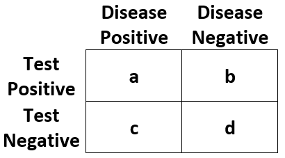
| Statistic | Abbreviation | Definition |
| Outcome Positive Rate | "pos_rate" | (a + c) / (a + b + c + d) |
| Outcome Negative Rate | "neg_rate" | (b + d) / (a + b + c + d) |
| Test Positive Rate | "test_pos_rate" | (a + b) / (a + b + c + d) |
| Test Negative Rate | "test_neg_rate" | (c + d) / (a + b + c + d) |
| True Positive Rate | "tp_rate" | a / (a + b + c + d) |
| False Positive Rate | "fp_rate" | b / (a + b + c + d) |
| False Negative Rate | "fn_rate" | c / (a + b + c + d) |
| True Negative Rate | "tn_rate" | d / (a + b + c + d) |
| Positive Predictive Value | "ppv" | a / (a + b) |
| Negative Predictive Value | "npv" | d / (c + d) |
| Sensitivity | "sens" | a / (a + c) |
| Specificity | "spec" | d / (b + d) |
| Positive Likelihood Ratio | "lr_pos" | sens / (1 - spec) |
| Negative Likelihood Ratio | "lr_neg" | (1 - sens) / spec |
Examples
test_consequences(cancer ~ cancerpredmarker, data = df_binary)