| Type: | Package |
| Title: | Causal Modeling with Coincidence Analysis |
| Version: | 4.0.3 |
| Date: | 2025-06-02 |
| Description: | Provides comprehensive functionalities for causal modeling with Coincidence Analysis (CNA), which is a configurational comparative method of causal data analysis that was first introduced in Baumgartner (2009) <doi:10.1177/0049124109339369>, and generalized in Baumgartner & Ambuehl (2020) <doi:10.1017/psrm.2018.45>. CNA is designed to recover INUS-causation from data, which is particularly relevant for analyzing processes featuring conjunctural causation (component causation) and equifinality (alternative causation). CNA is currently the only method for INUS-discovery that allows for multiple effects (outcomes/endogenous factors), meaning it can analyze common-cause and causal chain structures. Moreover, as of version 4.0, it is the only method of its kind that provides measures for model evaluation and selection that are custom-made for the problem of INUS-discovery. |
| License: | GPL-2 | GPL-3 [expanded from: GPL (≥ 2)] |
| URL: | https://CRAN.R-project.org/package=cna |
| Depends: | R (≥ 4.1.0) |
| Imports: | Rcpp, utils, stats, Matrix, matrixStats, car |
| LinkingTo: | Rcpp |
| Suggests: | dplyr, frscore, causalHyperGraph |
| NeedsCompilation: | yes |
| LazyData: | yes |
| Maintainer: | Mathias Ambuehl <mathias.ambuehl@consultag.ch> |
| Author: | Mathias Ambuehl [aut, cre, cph], Michael Baumgartner [aut, cph], Ruedi Epple [ctb], Veli-Pekka Parkkinen [ctb], Alrik Thiem [ctb] |
| Packaged: | 2025-06-02 05:28:52 UTC; MAM |
| Repository: | CRAN |
| Date/Publication: | 2025-06-02 06:30:02 UTC |
cna: A Package for Causal Modeling with Coincidence Analysis
Description
Coincidence Analysis (CNA) is a configurational comparative method of causal data analysis that was first introduced for crisp-set (i.e. binary) data in Baumgartner (2009a, 2009b, 2013) and generalized for multi-value and fuzzy-set data in Baumgartner and Ambuehl (2020). The cna package implements the method's latest stage of development.
CNA infers causal structures as defined by modern variants of the so-called INUS-theory (Mackie 1974; Grasshoff and May 2001; Baumgartner and Falk 2023a) from empirical data. The INUS-theory is a type-level difference-making theory that spells out causation in terms of redundancy-free Boolean dependency structures. It is optimally suited for the analysis of causal structures with the following features: conjunctivity—causes are arranged in complex bundles that only become operative when all of their components are properly co-instantiated, each of which in isolation is ineffective or leads to different outcomes—and disjunctivity—effects can be brought about along alternative causal routes such that, when suppressing one route, the effect may still be produced via another one.
Causal structures featuring conjunctivity and disjunctivity pose challenges for
methods of causal data analysis. As many theories of causation (other than the INUS-theory) entail that it is necessary (though not sufficient) for X to be a cause of Y that there be some kind of dependence (e.g. probabilistic or counterfactual) between X and Y, standard methods (e.g. Spirtes et al. 2000) infer that X is not a cause of Y if X and Y are not pairwise dependent.
However, there often are no dependencies between an individual component X of a conjunctive cause and the corresponding effect Y (for concrete examples see the package vignette (accessed from R by typing vignette("cna")). In the absence of pairwise dependencies, X can only be identified as a cause of Y if it is embedded in a complex Boolean structure over many factors and that structure is fitted to the data as a whole. But the space of Boolean functions over even a handful of factors is vast. So, a method for INUS-discovery must find ways to efficiently navigate in that vast space of possibilities. That is the purpose of CNA.
CNA is not the only method for the discovery of INUS structures. Other methods that can be used for that purpose are Logic Regression (Ruczinski et al. 2003, Kooperberg and Ruczinski 2005), which is implemented in the R package LogicReg, and Qualitative Comparative Analysis (Ragin 1987; 2008; Cronqvist and Berg-Schlosser 2009), whose most powerful implementations are provided by the R packages QCApro and QCA. But CNA is the only method for INUS-discovery that can process data generated by causal structures with more than one outcome and, hence, can analyze common-cause and causal chain structures as well as causal cycles and feedbacks. Moreover, as of version 4.0 of the cna package, it is the only method of its kind that offers measures for model evaluation and selection that are custom-made for the problem of INUS-discovery. Finally, unlike the models produced by Logic Regression or Qualitative Comparative Analysis, CNA's models are guaranteed to be redundancy-free, which makes them directly causally interpretable in terms of the INUS-theory; and CNA is more successful than any other method at exhaustively uncovering all INUS models that fit the data equally well. For comparisons of CNA with Qualitative Comparative Analysis and Logic Regression see (Baumgartner and Ambuehl 2020; Swiatczak 2022) and (Baumgartner and Falk 2023b), respectively.
There exist three additional R packages for data analysis with CNA: frscore, which automatizes robustness scoring of CNA models, causalHyperGraph, which visualizes CNA models as causal graphs, and cnaOpt, which systematizes the search for optimally fitting CNA models.
Details
| Package: | cna |
| Type: | Package |
| Version: | 4.0.3 |
| Date: | 2025-06-02 |
| License: | GPL (>= 2) |
Author(s)
Authors:
Mathias Ambuehl
mathias.ambuehl@consultag.ch
Michael Baumgartner
Department of Philosophy
University of Bergen
michael.baumgartner@uib.no
Maintainer:
Mathias Ambuehl
References
Baumgartner, Michael. 2009a. “Inferring Causal Complexity.” Sociological Methods & Research 38(1):71-101. doi:10.1177/0049124109339369
Baumgartner, Michael. 2009b. “Uncovering Deterministic Causal Structures: A Boolean Approach.” Synthese 170(1):71-96.
Baumgartner, Michael. 2013. “Detecting Causal Chains in Small-n Data.” Field Methods 25 (1):3-24. doi:10.1177/1525822X12462527
Baumgartner, Michael and Mathias Ambuehl. 2020. “Causal Modeling with Multi-Value and Fuzzy-Set Coincidence Analysis.” Political Science Research and Methods. 8:526-542. doi:10.1017/psrm.2018.45
Baumgartner, Michael and Christoph Falk. 2023a. “Boolean Difference-Making: A Modern Regularity Theory of Causation.” The British Journal for the Philosophy of Science, 74(1), 171-197. doi:10.1093/bjps/axz047
Baumgartner Michael and Christoph Falk. 2023b. “Configurational Causal Modeling and Logic Regression.” Multivariate Behavioral Research, 58:2, 292-310. doi:10.1080/00273171.2021.1971510
Cronqvist, Lasse, Dirk Berg-Schlosser. 2009. “Multi-Value QCA (mvQCA).” In B Rihoux, CC Ragin (eds.), Configurational Comparative Methods: Qualitative Comparative Analysis (QCA) and Related Techniques, pp. 69-86. Sage Publications, London.
Grasshoff, Gerd and Michael May. 2001. “Causal Regularities.” In W. Spohn, M. Ledwig, and M. Esfeld (Eds.). Current Issues in Causation, pp. 85-114. Paderborn: Mentis.
Mackie, John L. 1974. The Cement of the Universe: A Study of Causation. Oxford: Oxford University Press.
Kooperberg, Charles and Ingo Ruczinski. 2005. “Identifying Interacting SNPs Using Monte Carlo Logic Regression.” Genetic Epidemiology, 28(2):157-170.doi:10.1002/gepi.20042
Ragin, Charles C. 1987. The Comparative Method. Berkeley: University of California Press.
Ragin, Charles C. 2008. Redesigning Social Inquiry: Fuzzy Sets and Beyond. Chicago: University of Chicago Press.
Ruczinski, Ingo, Charles Kooperberg, and Michael LeBlanc. 2003. “Logic Regression.” Journal of Computational and Graphical Statistics 12:475-511. doi:10.1198/1061860032238
Spirtes, Peter, Clark Glymour, and Richard Scheines. 2000. “Causation, Prediction, and Search.” 2 edition. MIT Press, Cambridge.
Swiatczak, Martyna. 2022. “Different Algorithms, Different Models.” Quality & Quantity 56:1913-1937.
Perform Coincidence Analysis
Description
The cna function performs Coincidence Analysis to identify atomic solution formulas (asf) consisting of minimally necessary disjunctions of minimally sufficient conditions of all outcomes in the data
and combines the recovered asf to complex solution formulas (csf) representing multi-outcome structures, e.g. common-cause and/or causal chain structures.
Usage
cna(x, outcome = TRUE, con = 1, cov = 1, maxstep = c(3, 4, 10),
    measures = c("standard consistency", "standard coverage"),
    ordering = NULL, strict = FALSE, exclude = character(0), notcols = NULL,
    what = if (suff.only) "m" else "ac", details = FALSE,
    suff.only = FALSE, acyclic.only = FALSE, cycle.type = c("factor", "value"),
    verbose = FALSE, control = NULL, ...)
Arguments
x |
Data frame or |
outcome |
Character vector specifying one or several factor values that are to be considered as potential outcome(s). For crisp- and fuzzy-set data, factor values are expressed by upper and lower cases, for multi-value data, they are expressed by the "factor=value" notation.
Defaults to |
con |
Numeric scalar between 0 and 1 to set the threshold for the sufficiency measure selected in |
cov |
Numeric scalar between 0 and 1 to set the threshold for the necessity measure selected in |
maxstep |
Vector of three integers; the first specifies the maximum number of conjuncts in each disjunct of an asf, the second specifies the maximum number of disjuncts in an asf, the third specifies the maximum complexity of an asf. The complexity of an asf is
the total number of exogenous factor value appearances in the asf. Default: |
measures |
Character vector of length 2. |
ordering |
Character string or list of character vectors specifying the causal ordering of
the factors in |
strict |
Logical; if |
exclude |
Character vector specifying factor values to be excluded as possible causes of certain outcomes. For instance, |
notcols |
Character vector of factors to be negated in |
what |
Character string specifying what to print; |
details |
A character vector specifying the evaluation measures and additional solution attributes to be computed. Possible elements are all the measures in |
suff.only |
Logical; if |
acyclic.only |
Logical; if |
cycle.type |
Character string specifying what type of cycles to be detected: |
verbose |
Logical; if |
control |
Argument for fine-tuning and modifying the CNA algorithm (in ways that are not relevant for the ordinary user). See |
... |
Arguments for fine-tuning; passed to |
Details
The first input x of the cna function is a data frame or a configuration table. The data can be crisp-set (cs), fuzzy-set (fs), or multi-value (mv). Factors in cs data can only take values from {0,1}, factors in fs data can take on any (continuous) values from the unit interval [0,1], while factors in mv data can take on any of an open (but finite) number of non-negative integers as values. To ensure that no misinterpretations of returned asf and csf can occur, users are advised to exclusively use upper case letters as factor (column) names. Column names may contain numbers, but the first sign in a column name must be a letter. Only ASCII signs should be used for column and row names.
A data frame or configuration table x is the sole mandatory input of the cna function. In particular, cna does not need an input specifying which factor(s) in x are endogenous, it tries to infer that from the data. But if it is known prior to the analysis what factors have values that can figure as outcomes, an outcome specification can be passed to cna via the argument outcome, which takes as input a character vector identifying one or several factor values as potential outcome(s). For cs and fs data, outcomes are expressed by upper and lower cases (e.g. outcome = c("A", "b")). If factor names have multiple letters, any upper case letter is interpreted as 1, and the absence of upper case letters as 0 (i.e. outcome = c("coLd", "shiver") is interpreted as COLD=1 and SHIVER=0). For mv data, factor values are assigned by the “factor=value” notation (e.g. outcome = c("A=1","B=3")). Defaults to outcome = TRUE, which means that all factor values in x are potential outcomes.
When the data x contain multiple potential outcomes, it may moreover be known, prior to the analysis, that these outcomes have a certain causal ordering, meaning that some of them are causally upstream of the others. Such information can be passed to cna by means of the argument ordering, which takes either a character string or a list of character vectors as value. For example, ordering = "A, B < C" or, equivalently, ordering = list(c("A", "B"), "C") determines that factor C is causally located downstream of factors A and B, meaning that no values of C are potential causes of values of A and B. In consequence, cna only checks whether values of A and B can be modeled as causes of values of C; the test for a causal dependency in the other direction is skipped.
An ordering does not need to explicitly mention all factors in x. If only a subset of the factors are included in the ordering, the non-included factors are entailed to be upstream of the included ones. Hence, ordering = "C" means that C is located downstream of all other factors in x.
The argument strict determines whether the elements of one level in an ordering can be causally related or not. For example, if ordering = "A, B < C" and strict = TRUE, then the values of A and B—which are on the same level of the ordering—are excluded to be causally related and cna skips corresponding tests. By contrast, if ordering = "A, B < C" and strict = FALSE, then cna also searches for dependencies among the values of A and B. The default is strict = FALSE.
An ordering excludes all values of a factor as potential causes of an outcome. But a user may only be in a position to exclude some (not all) values as potential causes. Such information can be passed to cna through the argument exclude, which can be assigned a vector of character strings featuring the factor values to be excluded as causes to the left of the "->" sign and the corresponding outcomes on the right. For example, exclude = "A=1,C=3 -> B=1" determines that the value 1 of factor A and the value 3 of factor C are excluded as causes of the value 1 of factor B. Factor values can be excluded as potential causes of multiple outcomes as follows: exclude = c("A,c -> B", "b,H -> D"). For cs and fs data, upper case letters are interpreted as 1, lower case letters as 0. If factor names have multiple letters, any upper case letter is interpreted as 1, and the absence of upper case letters as 0. For mv data, the "factor=value" notation is required.
To exclude all values of a factor as potential causes of an outcome or to exclude a factor value as potential cause of all values of some endogenous factor, a "*" can be appended to the corresponding factor name; for example: exclude = "A* -> B" or exclude = "A=1,C=3 -> B*".
The exclude argument can be used both independently of and in conjunction with outcome and ordering, but if assignments to outcome and ordering contradict assignments to exclude, the latter are ignored. If exclude is assigned values of factors that do not appear in the data x, an error is returned.
If no outcomes are specified and no causal ordering is provided, all factor values in x are treated as potential outcomes; more specifically, in case of cs and fs data, cna tests for all factors whether their presence (i.e. them taking the value 1) can be modeled as an outcome, and in case of mv data, cna tests for all factors whether any of their possible values can be modeled as an outcome. That is done by searching for redundancy-free Boolean functions (in disjunctive normal form) that account for the behavior of an outcome in accordance with exclude.
The core Boolean dependence relations exploited for that purpose are sufficiency and necessity. To assess whether the (typically noisy) data warrant inferences to sufficiency and necessity, cna draws on evaluation measures for sufficiency and necessity, which can be selected via the argument measures, expecting a character vector of length 2. The first element, measures[1], specifies the measure to be used for sufficiency evaluation, and measures[2] specifies the measure to be used for necessity evaluation. All eight available evaluation measures can be printed to the console through showConCovMeasures. Four of them are sufficiency measures—variants of consistency (Ragin 2006)—, and four are necessity measures—variants of coverage (Ragin 2006). They implement different approaches for assessing whether the evidence in the data justifies an inference to sufficiency or necessity, respectively (cf. De Souter 2024; De Souter & Baumgartner 2025). The default is measures = c("standard consistency", "standard coverage"). More details are provided in section 3.2 of the cna package vignette (call vignette("cna")).
Against that background, cna first identifies, for each potential outcome in x, all minimally sufficient conditions (msc) that meet the threshold given to the selected sufficiency measure in the argument con. Then, these msc are disjunctively combined to minimally necessary conditions that meet the threshold for the selected necessity measure given to the argument cov, such that the whole disjunction meets con. The default value for con and cov is 1. The expressions resulting from this procedure are the atomic solution formulas (asf) for every factor value that can be modeled as an outcome. Asf represent causal structures with one outcome. To model structures with more than one outcome, the recovered asf are conjunctively combined to complex solution formulas (csf). To build its models, cna uses a bottom-up search algorithm, which we do not reiterate here (see Baumgartner and Ambuehl 2020 or the section 4 of vignette("cna")).
As the combinatorial search space of this algorithm is often too large to be exhaustively scanned in reasonable time, the argument maxstep allows for setting an upper bound for the complexity of the generated asf. maxstep takes a vector of three integers c(i, j, k) as input, entailing that the generated asf have maximally j disjuncts with maximally i conjuncts each and a total of maximally k factor value appearances (k is the maximal complexity). The default is maxstep = c(3, 4, 10).
Note that when the data x feature noise, the default con and cov thresholds of 1 will often not yield any asf. In such cases, con and cov may be set to values below 1. con and cov should neither be set too high, in order to avoid overfitting, nor too low, in order to avoid underfitting. The overfitting danger is severe in causal modeling with CNA (and configurational causal modeling more generally). For a discussion of this problem see Parkkinen and Baumgartner (2023), who also introduce a procedure for robustness assessment that explores all threshold settings in a given interval—in an attempt to reduce both over- and underfitting. See also the R package frscore.
If verbose is set to its non-default value TRUE, some information about the progression of the algorithm is returned to the console during the execution of the cna function. The execution can easily be interrupted by ESC at all stages.
The default output of cna first lists the provided ordering (if any), second, the pre-identified outcomes (if any), third, the implemented sufficiency and necessity measures, fourth, the recovered asf, and fifth, the csf. Asf and csf are ordered by complexity and the product of their con and cov scores.
For asf and csf, three attributes are standardly computed: con, cov, and complexity. The first two correspond to a solution's scores on the selected sufficiency and necessity measures, and the complexity score amounts to the number of factor value appearances on the left-hand sides of “->” or “<->” in asf and csf.
Apart from the evaluation measures used for model building through the measures argument, cna can also return the solution scores on all other available evaluation measures. This is accomplished by giving the details argument a character vector containing the names or aliases of the evaluation measures to be computed. For example, if details = c("ccon", "ccov", "PAcon", "AAcov"), the output of cna contains additional columns presenting the scores of the solutions on the requested measures.
In addition to measures evaluating the evidence for sufficiency and necessity, cna can calculate a number of further solution attributes: exhaustiveness, faithfulness, coherence, and cyclic all of which are recovered by requesting them through the details argument. Explanations of these attributes can be found in sections 5.2 to 5.4 of vignette("cna").
The argument notcols is used to calculate asf and csf
for negative outcomes in data of type cs and fs (in mv data notcols has no meaningful interpretation and, correspondingly, issues an error message). If notcols = "all", all factors in x are negated,
i.e. their membership scores i are replaced by 1-i. If notcols is given a character vector
of factors in x, only the factors in that vector are negated. For example, notcols = c("A", "B")
determines that only factors A and B are negated. The default is no negations, i.e. notcols = NULL.
suff.only is applicable whenever a complete cna analysis cannot be performed for reasons of computational complexity. In such a case, suff.only = TRUE forces cna to stop the analysis after the identification of msc, which will normally yield results even in cases when a complete analysis does not terminate. In that manner, it is possible to shed at least some light on the dependencies among the factors in x, in spite of an incomputable solution space.
The argument control provides a number of options to fine-tune and modify the CNA algorithm and the output of cna. It expects a list generated by the function cnaControl as input, for example, control = cnaControl(inus.only = FALSE, inus.def = c("equivalence"), con.msc = 0.8). The available fine-tuning parameters are documented here: cnaControl. All of the arguments in cnaControl can also be passed to the cna function directly via .... They all have default values yielding the standard behavior of cna, which do not have to be changed by the ordinary CNA user.
The argument what regulates what items of the output of cna are printed. It has no effect on the computations that are performed when executing cna; it only determines how the result is printed. See print.cna for more information on what.
Value
cna returns an object of class “cna”, which amounts to a list with the following elements:
call: | the executed function call |
x: | the processed data frame or configuration table, as input to cna |
ordering | the ordering imposed on the factors in the configuration table (if not NULL) |
configTable: | a “configTable” containing the the input data |
solution: | the solution object, which itself is composed of lists exhibiting msc and asf for all |
| outcome factors | |
measures: | the evaluation con- and cov-measures used for model-building |
what: | the values given to the what argument |
...: | plus additional list elements conveying more details on the function call and the |
| performed coincidence analysis. |
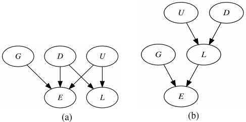
Note
In the first example described below (in Examples), the two resulting complex solution formulas represent a common cause structure and a causal chain, respectively. The common cause structure is graphically depicted in figure (a) below, the causal chain in figure (b).
References
Aleman, Jose. 2009. “The Politics of Tripartite Cooperation in New Democracies: A Multi-level Analysis.” International Political Science Review 30 (2):141-162.
Basurto, Xavier. 2013. “Linking Multi-Level Governance to Local Common-Pool Resource Theory using Fuzzy-Set Qualitative Comparative Analysis: Insights from Twenty Years of Biodiversity Conservation in Costa Rica.” Global Environmental Change 23(3):573-87.
Baumgartner, Michael. 2009. “Inferring Causal Complexity.” Sociological Methods & Research 38(1):71-101.
Baumgartner, Michael and Mathias Ambuehl. 2020. “Causal Modeling with Multi-Value and Fuzzy-Set Coincidence Analysis.” Political Science Research and Methods. 8:526–542.
Baumgartner, Michael and Christoph Falk. 2023. “Boolean Difference-Making: A Modern Regularity Theory of Causation.” The British Journal for the Philosophy of Science, 74(1), 171-197. doi:10.1093/bjps/axz047.
De Souter, Luna. 2024. “Evaluating Boolean Relationships in Configurational ComparativeMethods.” Journal of Causal Inference 12(1). doi:10.1515/jci-2023-0014.
De Souter, Luna and Michael Baumgartner. 2025. “New sufficiency and necessity measures for model building with Coincidence Analysis.” Zenodo. https://doi.org/10.5281/zenodo.13619580
Hartmann, Christof, and Joerg Kemmerzell. 2010. “Understanding Variations in Party Bans in Africa.” Democratization 17(4):642-65.
Krook, Mona Lena. 2010. “Women's Representation in Parliament: A Qualitative Comparative Analysis.” Political Studies 58(5):886-908.
Mackie, John L. 1974. The Cement of the Universe: A Study of Causation. Oxford: Oxford University Press.
Parkkinen, Veli-Pekka and Michael Baumgartner. 2023. “Robustness and Model Selection in Configurational Causal Modeling.” Sociological Methods & Research, 52(1), 176-208.
Ragin, Charles C. 2006. “Set Relations in Social Research: Evaluating Their Consistency and Coverage.” Political Analysis 14(3):291-310.
Wollebaek, Dag. 2010. “Volatility and Growth in Populations of Rural Associations.” Rural Sociology 75:144-166.
See Also
print.cna, configTable, condition, cyclic, condTbl, selectCases, makeFuzzy, some,
randomConds, is.submodel, is.inus, showMeasures, redundant, full.ct, d.educate,
d.women,
d.pban,d.autonomy, d.highdim
Examples
# Ideal crisp-set data from Baumgartner (2009) on education levels in western democracies
# ----------------------------------------------------------------------------------------
# Exhaustive CNA without constraints on the search space; print atomic and complex
# solution formulas (default output).
cna.educate <- cna(d.educate)
cna.educate
# The two resulting complex solution formulas represent a common cause structure
# and a causal chain, respectively. The common cause structure is graphically depicted
# in (Note, figure (a)), the causal chain in (Note, figure (b)).

# Build solutions with other than standard evaluation measures.
cna(d.educate, measures = c("ccon", "ccov"))
cna(d.educate, measures = c("PAcon", "PACcov"))

# CNA with negations of the factors E and L.
cna(d.educate, notcols = c("E","L"))
# The same by use of the outcome argument.
cna(d.educate, outcome = c("e","l"))

# CNA with negations of all factors.
cna(d.educate, notcols = "all")

# Print msc, asf, and csf with additional evaluation measures and solution attributes.
cna(d.educate, what = "mac", details = c("ccon","ccov","PAcon","PACcov","exhaustive"))
cna(d.educate, what = "mac", details = c("e","f","AACcon","AAcov"))
cna(d.educate, what = "mac", details = TRUE)

# Print solutions without spaces before and after "+".
options(spaces = c("<->", "->" ))
cna(d.educate, details = c("e", "f"))

# Print solutions with spaces before and after "*".
options(spaces = c("<->", "->", "*" ))
cna(d.educate, details = c("e", "f", "PAcon", "PACcov"))

# Restore the default of the option "spaces".
options(spaces = c("<->", "->", "+"))


# Crisp-set data from Krook (2010) on representation of women in western-democratic
# parliaments
# -----------------------------------------------------------------------------------
# This example shows that CNA can distinguish exogenous and endogenous factors in the
# data. Without being told which factor is the outcome, CNA reproduces the original
# QCA of Krook (2010).
ana1 <- cna(d.women, measures = c("PAcon", "PACcov"), details = c("e", "f"))
ana1

# The two resulting asf only reach an exhaustiveness score of 0.438, meaning that
# not all configurations that are compatible with the asf are contained in the data
# "d.women". Here is how to extract the configurations that are compatible with
# the first asf but are not contained in "d.women".
library(dplyr)
setdiff(ct2df(selectCases(asf(ana1)$condition[1], full.ct(d.women))),
        d.women)


# Highly ambiguous crisp-set data from Wollebaek (2010) on very high volatility of
# grassroots associations in Norway
# --------------------------------------------------------------------------------
# csCNA with ordering from Wollebaek (2010) [Beware: due to massive ambiguities,
# this analysis will take about 20 seconds to compute.]
cna(d.volatile, ordering = "VO2", maxstep = c(6, 6, 16))

# Using suff.only, CNA can be forced to abandon the analysis after minimization of
# sufficient conditions. [This analysis terminates quickly.]
cna(d.volatile, ordering = "VO2", maxstep = c(6, 6, 16), suff.only = TRUE)

# Similarly, by using the default maxstep, CNA can be forced to only search for asf
# and csf with reduced complexity.
cna(d.volatile, ordering = "VO2")

# ordering = "VO2" only excludes that the values of VO2 are causes of the values
# of the other factors in d.volatile, but cna() still tries to model other factor
# values as outcomes. The following call determines that only VO2 is a possible
# outcome. (This call terminates quickly.)
cna(d.volatile, outcome = "VO2")

# We can even increase maxstep.
cna(d.volatile, outcome = "VO2", maxstep=c(4,4,16))

# If it is known that, say, el and od cannot be causes of VO2, we can exclude this.
cna(d.volatile, outcome = "VO2", maxstep=c(4,4,16), exclude = "el, od -> VO2")

# The verbose argument returns information during the execution of cna().
cna(d.volatile, ordering = "VO2", verbose = TRUE)


# Multi-value data from Hartmann & Kemmerzell (2010) on party bans in Africa
# ---------------------------------------------------------------------------
# mvCNA with an outcome specification taken from Hartmann & Kemmerzell
# (2010); standard coverage threshold at 0.95 (standard consistency threshold at 1),
# maxstep at c(6, 6, 10).
cna.pban <- cna(d.pban, outcome = "PB=1", cov = .95, maxstep = c(6, 6, 10),
                  what = "all")
cna.pban

# The previous function call yields a total of 14 asf and csf, only 5 of which are
# printed in the default output. Here is how to extract all 14 asf and csf.
asf(cna.pban)
csf(cna.pban)

# [Note that all of these 14 causal models reach better consistency and
# coverage scores than the one model Hartmann & Kemmerzell (2010) present in their
# paper, which they generated using the TOSMANA software, version 1.3.
# T=0 + T=1 + C=2 + T=1*V=0 + T=2*V=0 <-> PB=1]
condTbl("T=0 + T=1 + C=2 + T=1*V=0 + T=2*V=0 <-> PB = 1", d.pban)

# Extract all minimally sufficient conditions with further details.
msc(cna.pban, details = c("ccon", "ccov", "PAcon", "PACcov"))

# Alternatively, all msc, asf, and csf can be recovered by means of the nsolutions
# argument of the print function, which also allows for adding details.
print(cna.pban, nsolutions = "all", details = c("AACcon", "AAcov", "ex", "fa"))

# Print the configuration table with the "cases" column.
print(cna.pban, what = "t", show.cases = TRUE)

# Build solution formulas with maximally 4 disjuncts.
cna(d.pban, outcome = "PB=1", cov = .95, maxstep = c(4, 4, 10))

# Use non-standard evaluation measures for solution building.
cna(d.pban, outcome = "PB=1", cov = .95, measures = c("PAcon", "PACcov"))

# Only print 2 digits of standard consistency and coverage scores.
print(cna.pban, digits = 2)

# Build all but print only two msc for each factor and two asf and csf.
print(cna(d.pban, outcome = "PB=1", cov = .95,
          maxstep = c(6, 6, 10), what = "all"), nsolutions = 2)

# Lowering the thresholds on standard consistency and coverage yields further
# models with excellent fit scores; print only asf.
cna(d.pban, outcome = "PB=1", con = .93, what = "a", maxstep = c(6, 6, 10))

# Lowering both standard consistency and coverage.
cna(d.pban, outcome = "PB=1", con = .9, cov =.9, maxstep = c(6, 6, 10))

# Lowering both standard consistency and coverage and excluding F=0 as potential
# cause of PB=1.
cna(d.pban, outcome = "PB=1", con = .9, cov =.9, maxstep = c(6, 6, 10),
    exclude = "F=0 -> PB=1")

# Specifying an outcome is unnecessary for d.pban. PB=1 is the only
# factor value in those data that could possibly be an outcome.
cna(d.pban, con=.9, cov = .9, maxstep = c(6, 6, 10))


# Fuzzy-set data from Basurto (2013) on autonomy of biodiversity institutions in Costa Rica
# ---------------------------------------------------------------------------------------
# Basurto investigates two outcomes: emergence of local autonomy and endurance thereof. The
# data for the first outcome are contained in rows 1-14 of d.autonomy, the data for the second
# outcome in rows 15-30. For each outcome, the author distinguishes between local ("EM",
# "SP", "CO"), national ("CI", "PO") and international ("RE", "CN", "DE") conditions. Here,
# we first apply fsCNA to replicate the analysis for the local conditions of the endurance of
# local autonomy.
dat1 <- d.autonomy[15:30, c("AU","EM","SP","CO")]
cna(dat1, ordering = "AU", strict = TRUE, con = .9, cov = .9)

# The CNA model has significantly better consistency (and equal coverage) scores than the
# model presented by Basurto (p. 580): SP*EM + CO <-> AU, which he generated using the
# fs/QCA software.
condition("SP*EM + CO <-> AU", dat1) # both EM and CO are redundant to account for AU

# If we allow for dependencies among the conditions by setting strict = FALSE, CNA reveals
# that SP is a common cause of both AU and EM.
cna(dat1, ordering = "AU", strict = FALSE, con = .9, cov = .9)

# Here are two analyses at different con/cov thresholds for the international conditions
# of autonomy endurance.
dat2 <- d.autonomy[15:30, c("AU","RE", "CN", "DE")]
cna(dat2, ordering = "AU", con = .9,  cov = .85)
cna(dat2, ordering = "AU", con = .85, cov = .9, details = TRUE)

# Here are two analyses of the whole dataset using different evaluation measures.
# They show that across the whole period 1986-2006, the best causal model of local
# autonomy (AU) renders that outcome dependent only on local direct spending (SP).
cna(d.autonomy, outcome = "AU", con = .85, cov = .9,
    maxstep = c(5, 5, 11), details = TRUE)
cna(d.autonomy, outcome = "AU", measures = c("AACcon","AAcov"), con = .85, cov = .9,
    maxstep = c(5, 5, 11), details = TRUE)


# High-dimensional data
# ---------------------
# Here's an analysis of the data d.highdim with 50 factors, massive
# fragmentation, and 20% noise. (Takes about 15 seconds to compute.)
head(d.highdim)
cna(d.highdim,  outcome = c("V13", "V11"), con = .8, cov = .8)

# By lowering maxstep, computation time can be reduced to less than 1 second
# (at the cost of an incomplete solution).
cna(d.highdim,  outcome = c("V13", "V11"), con = .8, cov = .8,
    maxstep = c(2,3,10))


# Highly ambiguous artificial data to illustrate exhaustiveness and acyclic.only
# ------------------------------------------------------------------------------
mycond <- "(D + C*f <-> A)*(C*d + c*D <-> B)*(B*d + D*f <-> C)*(c*B + B*f <-> E)"
dat1 <- selectCases(mycond)
ana1 <- cna(dat1, details = c("e","cy"))
# There exist almost 2M csf. This is how to build the first 927 of them, with
# additional messages about the csf building process.
first.csf <- csf(ana1, verbose = TRUE)
first.csf
# Most of these csf are compatible with more configurations than are contained in
# dat1. Only 141 csf in first.csf are perfectly exhaustive (i.e. all compatible
# configurations are contained in dat1).
subset(first.csf, exhaustiveness == 1)

# All of the csf in first.csf contain cyclic substructures.
subset(first.csf, cyclic == TRUE)

# Here's how to build acyclic csf.
ana2 <- cna(dat1, details = c("e","cy"), acyclic.only = TRUE)
csf(ana2, verbose = TRUE)
Deprecated functions in the cna package
Description
These functions are provided for compatibility with older versions of the cna package only, and may be removed eventually. They have become obsolete since the introduction of the default setting type = "auto" in package version 3.2.0.
Usage
csct(...)
mvct(...)
fsct(...)

cscna(...)
mvcna(...)
fscna(...)

cscond(...)
mvcond(...)
fscond(...)
Arguments
... |
In |
Details
csct(x, ...), mvct(x, ...), and fsct(x, ...) are shorthands for configTable(x, type = "cs", ...), configTable(x, type = "mv", ...) and configTable(x, type = "fs", ...), respectively.
cscna(x, ...), mvcna(x, ...), and fscna(x, ...) are shorthands for cna(x, type = "cs", ...), cna(x, type = "mv", ...) and cna(x, type = "fs", ...), respectively.
cscond(x, ct, ...), mvcond(x, ct, ...), and fscond(x, ct, ...) are shorthands for condition(x, ct, type = "cs", ...), condition(x, ct, type = "mv", ...) and condition(x, ct, type = "fs", ...), respectively.
See Also
Internal functions in the cna package
Description
These functions are mainly for internal purposes and will not normally be called directly by the user.
Overview of Functions
noblanks,lhs,rhs,extract_asf:-
Manipulation of character vectors containing conditions and atomic solution formulas.
ctInfo:-
Alternative internal represenation of a
configTable. qcond_bool,qcond_asf,qcond_csf:-
Fast evaluation of the well-formedness of conditions, asf, and csf.
getCondType,getComplexity:-
Extract condition type and complexity values from a character vector containing conditions.
stdCond,matchCond:-
Standardize and match conditions.
relist1,hstrsplit,C_mconcat,C_mconcat,C_recCharList2char,C_relist_Int:-
Utility functions for conversion between different represenations of conditions.
C_redund:-
Internal version of the test for structural redundancy (used in
redundant). getCond:-
Derive a condition from a data set.
rreduce:-
Eliminate redundancies from a disjunctive normal form.
redundant,minimalizeCsf:-
Identify structurally redundant asf in a csf and eliminate them.
C_is_submodel:-
Internal core of the function
is.submodel. .det,.inus,.exff,.redund,.inCsf:-
These are generic auxiliary functions used internally within other functions.
Extract solutions from an object of class “cna”
Description
Given a solution object x produced by cna, msc(x) extracts all minimally sufficient conditions, asf(x) all atomic solution formulas, and csf(x, n.init) builds approximately n.init complex solution formulas. All solution attributes (details) available in showMeasures can be computed. The three functions return a data frame with the additional class attribute “condTbl”.
Usage
msc(x, details = x$details, cases = FALSE)
asf(x, details = x$details)
csf(x, n.init = 1000, details = x$details, asfx = NULL,
    inus.only = x$control$inus.only, inus.def = x$control$inus.def,
    minimalizeCsf = inus.only,
    acyclic.only = x$acyclic.only, cycle.type = x$cycle.type, verbose = FALSE)
Arguments
x |
Object of class “cna”. |
details |
A character vector specifying the evaluation measures and additional solution attributes to be computed. Possible elements are all the measures in |
cases |
Logical; if |
n.init |
Integer capping the amount of initial asf combinations. Default at 1000. Serves to control the computational complexity of the csf building process. |
asfx |
Object of class “condTbl” produced by the |
inus.only |
Logical; if |
inus.def |
Character string specifying the definition of partial structural redundancy to be applied. Possible values are "implication" or "equivalence". The strings can be abbreviated. Cf. also |
minimalizeCsf |
Logical; if |
acyclic.only |
Logical; if |
cycle.type |
Character string specifying what type of cycles to be detected: |
verbose |
Logical; if |
Details
Depending on the processed data, the solutions (models) output by cna are often ambiguous, to the effect that many atomic and complex solutions fit the data equally well. To facilitate the inspection of the cna output, however, cna standardly returns only 5 minimally sufficient conditions (msc) and 5 atomic solution formulas (asf) for each outcome as well as 5 complex solution formulas (csf). msc can be used to extract all msc from an object x of class “cna”, asf to extract all asf, and csf to build approximately n.init csf from the asf stored in x. All solution attributes (details) that are saved in x are recovered as well. Moreover, all evaluation measures and solution attributes available in showMeasures—irrespective of whether they are saved in x—can be computed by specifying them in the details argument.
The outputs of msc, asf, and csf can be further processed by the condition function.
While msc and asf merely extract information stored in x, csf builds csf from the inventory of asf recovered at the end of the third stage of the cna algorithm (cf. vignette("cna"), section 4). That is, the csf function implements the fourth stage of that algorithm. It proceeds in a stepwise manner as follows.
-
n.initpossible conjunctions featuring one asf of every outcome are built. If
inus.only = TRUEorminimalizeCsf = TRUE, the solutions resulting from step 1 are freed of structural redundancies (cf. Baumgartner and Falk 2023).If
inus.only = TRUE, tautologous and contradictory solutions as well as solutions with partial structural redundancies (as defined ininus.def) and constant factors are eliminated. [Ifinus.only = FALSEandminimalizeCsf = TRUE, only structural redundancies are eliminated, meaning only step 2, but not step 3, is executed.]If
acyclic.only = TRUE, solutions with cyclic substructures are eliminated.Solutions that are a submodel of another solution are removed.
For those solutions that were modified in the previous steps, the scores on the selected evaluation
measuresare re-calculated and solutions that no longer reachconorcovare eliminated (cf.cna).The remaining solutions are returned as csf, ordered by complexity and the product of their scores on the evaluation
measures.
Value
msc, asf and csf return objects of class “condTbl”, an object similar to a data.frame, which features the following components:
outcome: | the outcomes |
condition: | the relevant conditions or solutions |
con: | the scores on the sufficiency measure (e.g. consistency) |
cov: | the scores on the necessity measure (e.g. coverage) |
complexity: | the complexity scores (number of factor value appearances to the left of “<->”) |
...: | scores on additional evaluation measures and solution attributes as specified in |
details
|
References
Lam, Wai Fung, and Elinor Ostrom. 2010. “Analyzing the Dynamic Complexity of Development Interventions: Lessons from an Irrigation Experiment in Nepal.” Policy Sciences 43 (2):1-25.
See Also
cna, configTable, condition, condTbl, cnaControl, is.inus, detailMeasures, showMeasures, cyclic, d.irrigate
Examples
# Crisp-set data from Lam and Ostrom (2010) on the impact of development interventions
# ------------------------------------------------------------------------------------
# CNA with causal ordering that corresponds to the ordering in Lam & Ostrom (2010); coverage
# cut-off at 0.9 (consistency cut-off at 1).
cna.irrigate <- cna(d.irrigate, ordering = "A, R, F, L, C < W", cov = .9,
                    maxstep = c(4, 4, 12), details = TRUE)
cna.irrigate

# The previous function call yields a total of 12 complex solution formulas, only
# 5 of which are returned in the default output.
# Here is how to extract all 12 complex solution formulas along with all
# solution attributes.
csf(cna.irrigate)
# With only the used evaluation measures and complexity plus exhaustiveness and faithfulness.
csf(cna.irrigate, details = c("e", "f"))
# Calculate additional evaluation measures from showCovCovMeasures().
csf(cna.irrigate, details = c("e", "f", "PAcon", "PACcov", "AACcon", "AAcov"))

# Extract all atomic solution formulas.
asf(cna.irrigate, details = c("e", "f"))

# Extract all minimally sufficient conditions.
msc(cna.irrigate) # capped at 20 rows
print(msc(cna.irrigate), n = Inf) # prints all rows
# Add cases featuring the minimally sufficient conditions combined
# with the outcome.
(msc.table <- msc(cna.irrigate, cases = TRUE))
# Render as data frame.
as.data.frame(msc.table)

# Extract only the conditions (solutions).
csf(cna.irrigate)$condition
asf(cna.irrigate)$condition
msc(cna.irrigate)$condition

# A CNA of d.irrigate without outcome specification and ordering is even more
# ambiguous.
cna2.irrigate <- cna(d.irrigate, cov = .9, maxstep = c(4,4,12),
                     details = c("e", "f", "ccon", "ccov"))

# Reduce the initial asf combinations to 50.
csf(cna2.irrigate, n.init = 50)
# Print the first 20 csf.
csf(cna2.irrigate, n.init = 50)[1:20, ]

# Print details about the csf building process.
csf(cna.irrigate, verbose = TRUE)

# Return evaluation measures and solution attributes with 5 digits.
print(asf(cna2.irrigate), digits = 5)


# Further examples
# ----------------
# An example generating structural redundancies.
target <- "(A*B + C <-> D)*(c + a <-> E)"
dat1 <- selectCases(target)
ana1 <- cna(dat1, maxstep = c(3, 4, 10))
# Run csf with elimination of structural redundancies.
csf(ana1, verbose = TRUE)
# Run csf without elimination of structural redundancies.
csf(ana1, verbose = TRUE, inus.only = FALSE)

# An example generating partial structural redundancies.
dat2 <- data.frame(
  A=c(0,0,0,0,1,1,1,1,0,0,0,0,1,1,1,1,1,1,1,1,1,1,1,1,1,0, 1),
  B=c(0,0,1,1,0,0,0,0,0,0,1,0,0,0,0,0,0,0,0,0,0,0,0,0,0,1,1),
  C=c(1,1,0,0,0,1,0,0,1,1,0,1,1,0,1,1,0,1,1,1,0,1,0,1,0,1,0),
  D=c(0,1,1,1,0,1,1,1,0,0,0,1,0,1,0,0,0,1,0,0,0,1,1,0,0,1,0),
  E=c(1,0,0,0,0,1,1,1,1,1,1,0,0,1,0,0,0,1,1,1,1,0,0,0,0,1,1),
  F=c(1,1,1,1,1,0,0,0,0,0,0,0,0,1,1,1,1,0,0,0,0,0,0,0,0,0,0),
  G=c(1,1,1,1,1,1,1,1,1,1,1,1,1,0,0,0,0,0,0,0,0,0,0,0,0,1,1))
ana2 <- cna(dat2, con = .8, cov = .8, maxstep = c(3, 3, 10))
# Run csf without elimination of partial structural redundancies.
csf(ana2, inus.only = FALSE, verbose = TRUE)
# Run csf with elimination of partial structural redundancies.
csf(ana2, verbose = TRUE)
# Prior to version 3.6.0, the "equivalence" definition of partial structural
# redundancy was used by default (see ?is.inus() for details). Now, the
# "implication" definition is used. To replicate old behavior
# set inus.def to "equivalence".
csf(ana2, verbose = TRUE, inus.def = "equivalence")
# The two definitions only come apart in case of cyclic structures.
# Build only acyclic models.
csf(ana2, verbose = TRUE, acyclic.only = TRUE)
# Add further details.
csf(ana2, verbose = TRUE, acyclic.only = TRUE, details = c("PAcon", "PACcov"))
Fine-tuning and modifying the CNA algorithm
Description
The cnaControl function provides a number of arguments for fine-tuning and modifying the CNA algorithm as implemented in the cna function. The arguments can also be passed directly to the cna function. All arguments in cnaControl have default values that should be left unchanged for most CNA applications.
Usage
cnaControl(inus.only = TRUE, inus.def = c("implication","equivalence"),
           type = "auto", con.msc = NULL,
           rm.const.factors = FALSE, rm.dup.factors = FALSE,
           cutoff = 0.5, border = "up", asf.selection = c("cs", "fs", "none"),
           only.minimal.msc = TRUE, only.minimal.asf = TRUE, maxSol = 1e+06)
Arguments
inus.only |
Logical; if |
inus.def |
Character string specifying the definition of partial structural redundancy to be applied. Possible values are "implication" or "equivalence". The strings can be abbreviated. |
type |
Character vector specifying the type of the data analyzed by |
con.msc |
Numeric scalar between 0 and 1 to set the minimum threshold every msc must satisfy on the sufficiency measure selected in |
rm.const.factors, rm.dup.factors |
Logical; if |
cutoff |
Minimum membership score required for a factor to count as instantiated in the data and to be integrated into the analysis. Value in the unit interval [0,1]. The default cutoff is 0.5. Only meaningful if the data is fuzzy-set ( |
border |
Character string specifying whether factors with membership scores equal to |
asf.selection |
Character string specifying how to select asf based on outcome variation in configurations incompatible with a model. |
only.minimal.msc |
Logical; if |
only.minimal.asf |
Logical; if |
maxSol |
Maximum number of asf calculated. The default value should normally not be changed by the user. |
Details
When the inus.only argument takes its default value TRUE, the cna function only returns solution formulas—asf and csf—that are freed of all types of redundancies: redundancies in sufficient and necessary conditions as well as structural and partial structural redundancies. Moreover, tautologous and contradictory solutions and solutions featuring constant factors are eliminated (cf. is.inus). In other words, at inus.only = TRUE, cna issues so-called MINUS-formulas only (cf. vignette("cna") for details). MINUS-formulas are causally interpretable. In some research contexts, however, solution formulas with redundancies might be of interest, for example, when the analyst is not searching for causal models but for models with maximal data fit. In such cases, the inus.only argument can be set to its non-default value FALSE.
The notion of a partial structural redundancy (PSR) can be defined in two different ways, which can be selected through the inus.def argument. If inus.def = "implication" (default), a solution formula is treated as containing a PSR iff it logically implies a proper submodel of itself. If inus.def = "equivalence", a PSR obtains iff the solution formula is logically equivalent with a proper submodel of itself. The character string passed to inus.def can be abbreviated. To reproduce results produced by versions of the cna package prior to 3.6.0, inus.def may have to be set to "equivalence", which was the default in earlier versions.
The argument type allows for manually specifying the type of data passed to the cna function. The argument has the default value "auto", inducing automatic detection of the data type. But the user can still manually set the data type. Data with factors taking values 1 or 0 only are called crisp-set, which can be indicated by type = "cs". If the data contain at least one factor that takes more than two values, e.g. {1,2,3}, the data count as multi-value: type = "mv". Data featuring at least one factor taking real values from the interval [0,1] count as fuzzy-set: type = "fs". (Note that mixing multi-value and fuzzy-set factors in one analysis is not supported). One context in which users may want to set the data type manually is when they are interested in receiving models for both the presence and the absence of a crisp-set outcome from just one call of the cna function. When analyzing cs data x, cna(x, ordering = "A", type = "mv") searches for models of A=1 and A=0 at the same time, whereas the default cna(x, ordering = "A") searches for models of A=1 only.
The cna function standardly takes one threshold con for the selected sufficiency measure, e.g. consistency, that is imposed on both minimally sufficient conditions (msc) and solution formulas, asf and csf. But the analyst may want to impose a different con threshold on msc than on asf and csf. This can be accomplished by setting the argument con.msc to a different value than con. In that case, cna first builds msc using con.msc and then combines these msc to asf and to csf using con (and cov). See Examples below for a concrete context, in which this might be useful.
rm.const.factors and rm.dup.factors are used to determine the handling of constant factors, i.e. factors with constant values in all cases (rows) in the data analyzed by cna, and of duplicated factors, i.e. factors with identical value distributions in all cases in the data. If the arguments are given the value TRUE, factors with constant values are removed and all but the first of a set of duplicated factors are removed. As of package version 3.5.4, the default is FALSE for both rm.const.factors and rm.dup.factors, which means that constant and duplicated factors are not removed. See configTable for more details.
cna only includes factor configurations in the analysis that are actually instantiated in the data. The argument cutoff determines the minimum membership score required for a factor or a combination of factors to count as instantiated. It takes values in the unit interval [0,1] with a default of 0.5. border specifies whether configurations with membership scores equal to cutoff are rounded up (border = "up"), which is the default, or rounded down (border = "down").
If the data analyzed by cna feature noise, it can happen that all variation of an outcome occurs in noisy configurations in the data. In such cases, there may be asf that meet chosen con and cov thresholds (lower than 1) such that the corresponding outcome only varies in configurations that are incompatible with the strict crisp-set or fuzzy-set necessity and sufficiency relations expressed by those very asf. In the default setting "cs" of the argument asf.selection, an asf is only returned if the outcome takes a value above and below the 0.5 anchor in the configurations compatible with the strict crisp-set necessity and sufficiency relations expressed by that asf. At asf.selection = "fs", an asf is only returned if the outcome takes different values in the configurations compatible with the strict fuzzy-set necessity and sufficiency relations expressed by that asf. At asf.selection = "none", asf are returned even if outcome variation only occurs in noisy configurations. (For more details, see Examples below.)
To recover certain target structures from noisy data, it may be useful to allow cna to also consider sufficient conditions for further analysis that are not minimal (i.e. redundancy-free). This can be accomplished by setting only.minimal.msc to its non-default value FALSE. A concrete example illustrating the utility of only.minimal.msc = FALSE is provided in the Examples section below. Similarly, to recover certain target structures from noisy data, cna may need to also consider necessary conditions for further analysis that are not minimal. This is accomplished by setting only.minimal.asf to FALSE, in which case all disjunctions of msc reaching the con and cov thresholds will be returned. (The ordinary user is advised not to change the default values of either argument.)
For details on the usage of cnaControl, see the example below.
Value
A list of parameter settings.
See Also
cna, is.inus, configTable, showConCovMeasures
Examples
# cnaControl() generates a list that can be passed to the control argument of cna().
cna(d.jobsecurity, outcome = "JSR", con = .85, cov = .85, maxstep = c(3,3,9),
    control = cnaControl(inus.only = FALSE, only.minimal.msc = FALSE, con.msc = .78))
# The fine-tuning arguments can also be passed to cna() directly.
cna(d.jobsecurity, outcome = "JSR", con = .85, cov = .85, maxstep = c(3,3,9),
    inus.only = FALSE, only.minimal.msc = FALSE, con.msc = .78)
# Changing the set-inclusion cutoff and border rounding.
cna(d.jobsecurity, outcome = "JSR", con = .85, cov = .85,
  	control = cnaControl(cutoff= 0.6, border = "down"))
# Modifying the handling of constant factors.
data <- subset(d.highdim, d.highdim$V4==1)
cna(data, outcome = "V11", con=0.75, cov=0.75, maxstep = c(2,3,9),
		control = cnaControl(rm.const.factors = TRUE))


# Illustration of only.minimal.msc = FALSE
# ----------------------------------------
# Simulate noisy data on the causal structure "a*B*d + A*c*D <-> E"
set.seed(1324557857)
mydata <- allCombs(rep(2, 5)) - 1
dat1 <- makeFuzzy(mydata, fuzzvalues = seq(0, 0.5, 0.01))
dat1 <- ct2df(selectCases1("a*B*d + A*c*D <-> E", con = .8, cov = .8, dat1))

# In dat1, "a*B*d + A*c*D <-> E" has the following con and cov scores.
as.condTbl(condition("a*B*d + A*c*D <-> E", dat1))

# The standard algorithm of CNA will, however, not find this structure with
# con = cov = 0.8 because one of the disjuncts (a*B*d) does not meet the con
# threshold.
as.condTbl(condition(c("a*B*d <-> E", "A*c*D <-> E"), dat1))
cna(dat1, outcome = "E", con = .8, cov = .8)

# With the argument con.msc we can lower the con threshold for msc, but this does not
# recover "a*B*d + A*c*D <-> E" either.
cna2 <- cna(dat1, outcome = "E", con = .8, cov = .8, con.msc = .78)
cna2
msc(cna2)

# The reason is that "A*c -> E" and "c*D -> E" now also meet the con.msc threshold and,
# therefore,  "A*c*D -> E" is not contained in the msc---because of violated minimality.
# In a situation like this, lifting the minimality requirement via
# only.minimal.msc = FALSE allows CNA to find the intended target.
cna(dat1, outcome = "E", con = .8, cov = .8, control = cnaControl(con.msc = .78,
		only.minimal.msc = FALSE))


# Overriding automatic detection of the data type
# ------------------------------------------------
# The type argument allows for manually setting the data type.
# If "cs" data are treated as "mv" data, cna() automatically builds models for all values
# of outcome factors, i.e. both positive and negated outcomes.
cna(d.educate, control = cnaControl(type = "mv"))
# Treating "cs" data as "fs".
cna(d.women, type = "fs")

# Not all manual settings are admissible.
try(cna(d.autonomy, outcome = "AU", con = .8, cov = .8, type = "mv" ))


# Illustration of asf.selection
# -----------------------------
# Consider the following data set:
d1 <- data.frame(X1 = c(1, 0, 1),
				X2 = c(0, 1, 0),
				Y = c(1, 1, 0))
ct1 <- configTable(d1, frequency = c(10, 10, 1))

# Both of the following asf reach con=0.95 and cov=1.
condition(c("X1+X2<->Y", "x1+x2<->Y"), ct1)

# Up to version 3.4.0 of the cna package, these two asf were inferred from
# ct1 by cna(). But the outcome Y is constant in ct1, except for a variation in
# the third row, which is incompatible with X1+X2<->Y and x1+x2<->Y. Subject to
# both of these models, the third row of ct1 is a noisy configuration. Inferring
# difference-making models that are incapable of accounting for the only difference
# in the outcome in the data is inadequate. (Thanks to Luna De Souter for
# pointing out this problem.) Hence, as of version 3.5.0, asf whose outcome only
# varies in configurations incompatible with the strict crisp-set necessity
# or sufficiency relations expressed by those asf are not returned anymore.

cna(ct1, outcome = "Y", con = 0.9)

# The old behavior of cna() can be obtained by setting the argument asf.selection
# to its non-default value "none".

cna(ct1, outcome = "Y", con = 0.9, control = cnaControl(asf.selection = "none"))

# Analysis of fuzzy-set data from Aleman (2009).
cna(d.pacts, con = .9, cov = .85)
cna(d.pacts, con = .9, cov = .85, asf.selection = "none")
# In the default setting, cna() does not return any model for d.pacts because
# the outcome takes a value >0.5 in every single case, meaning it does not change
# between presence and absence. No difference-making model should be inferred from
# such data.
# The implications of asf.selection can also be traced by
# the verbose argument:

cna(d.pacts, con = .9, cov = .85, verbose = TRUE)
Calculate the coherence of complex solution formulas
Description
Calculates the coherence measure of complex solution formulas (csf).
Usage
coherence(x, ...)
## Default S3 method:
coherence(x, ct, type, ...)
Arguments
x |
Character vector specifying an asf or csf. |
ct |
Data frame or |
type |
Character vector specifying the type of |
... |
Arguments passed to methods. |
Details
Coherence is a measure for model fit that is custom-built for complex solution formulas (csf). It measures the degree to which the atomic solution formulas (asf) combined in a csf cohere, i.e. are instantiated together in x rather than independently of one another. More concretely, coherence is the ratio of the number of cases satisfying all asf contained in a csf to the number of cases satisfying at least one asf in the csf. For example, if the csf contains the three asf asf1, asf2, asf3, coherence amounts to | asf1 * asf2 * asf3 | / | asf1 + asf2 + asf3 |, where |...| expresses the cardinality of the set of cases in x instantiating the corresponding expression. For asf, coherence returns 1. For boolean conditions (see condition), the coherence measure is not defined and coherence hence returns NA. For multiple csf that do not have a factor in common, coherence returns the minimum of the separate coherence scores.
Value
Numeric vector of coherence values to which cond is appended as a "names" attribute. If cond is a csf "asf1*asf2*asf3" composed of asf that do not have a factor in common, the csf is rendered with commas in the "names" attribute: "asf1, asf2, asf3".
See Also
cna, condition, selectCases, configTable, allCombs, full.ct, condTbl
Examples
# Perfect coherence.
dat1 <- selectCases("(A*b <-> C)*(C + D <-> E)")
coherence("(A*b <-> C)*(C + D <-> E)", dat1)
csf(cna(dat1, details = "coherence"))

# Non-perfect coherence.
dat2 <- selectCases("(a*B <-> C)*(C + D <-> E)*(F*g <-> H)")
dat3 <- rbind(ct2df(dat2), c(0,1,0,1,1,1,0,1))
coherence("(a*B <-> C)*(C + D <-> E)*(F*g <-> H)", dat3)
csf(cna(dat3, con = .88, details = "coherence"))
Methods for class “condList”
Description
The output of the condition (aka condList) function is a nested list of class “condList” that contains one or several data frames. The utilities in condList-methods are suited for rendering or reshaping these objects in different ways.
Usage
## S3 method for class 'condList'
summary(object, n = 6, ...)

## S3 method for class 'condList'
as.data.frame(x, row.names = attr(x, "cases"), optional = TRUE, nobs = TRUE, ...)

group.by.outcome(object, cases = TRUE)
Arguments
object, x |
Object of class “condList” as output by the |
n |
Positive integer: the maximal number of conditions to be printed. |
... |
Not used. |
row.names, optional |
As in |
nobs |
Logical; if |
cases |
Logical; if |
Details
The summary method for class “condList” prints the output of condition in a condensed manner. It is identical to printing with print.table = FALSE (but with a different default of argument n), see print.condList.
The output of condition is a nested list of class “condList” that contains one or several data frames. The method as.data.frame is a variant of the base method as.data.frame. It offers a convenient way of combining the columns of the data frames in a condList into one regular data frame.
Columns appearing in several tables (typically the modeled outcomes) are included only once in the resulting data frame. The output of as.data.frame has syntactically invalid column names by default, including operators such as "->" or "+".
Setting optional = FALSE converts the column names into syntactically valid names (using make.names).
group.by.outcome takes a condList as input and combines the entries in that nested list into a data frame with a larger number of columns, combining all columns concerning the same outcome into the same data frame. The additional attributes (measures, info, etc.) are thereby removed.
See Also
condition, condList, as.data.frame, make.names
Examples
# Analysis of d.irrigate data with standard evaluation measures.
ana1 <- cna(d.irrigate, ordering = "A, R, L < F, C < W", con = .9)
(ana1.csf <- condition(csf(ana1)$condition, d.irrigate))
# Convert condList to data frame.
as.data.frame(ana1.csf)
as.data.frame(ana1.csf[1]) # Include the first condition only
as.data.frame(ana1.csf, row.names = NULL)
as.data.frame(ana1.csf, optional = FALSE)
as.data.frame(ana1.csf, nobs = FALSE)
# Summary.
summary(ana1.csf)
# Analyze atomic solution formulas.
(ana1.asf <- condition(asf(ana1)$condition, d.irrigate))
as.data.frame(ana1.asf)
summary(ana1.asf)
# Group by outcome.
group.by.outcome(ana1.asf)
# Analyze minimally sufficient conditions.
(ana1.msc <- condition(msc(ana1)$condition, d.irrigate))
as.data.frame(ana1.msc)
group.by.outcome(ana1.msc)
summary(ana1.msc)
# Print more than 6 conditions.
summary(ana1.msc, n = 10)

# Analysis with different evaluation measures.
ana2 <- cna(d.irrigate, ordering = "A, R, L < F, C < W", con = .9, cov = .9,
            measures = c("PAcon", "PACcov"))
(ana2.csf <- condition(csf(ana2)$condition, d.irrigate))
print(ana2.csf, add.data = d.irrigate, n=10)
as.data.frame(ana2.csf, nobs = FALSE, row.names = NULL)
summary(ana2.csf, n = 10)
Create summary tables for conditions
Description
The function condTbl returns a table of class “condTbl”, which is a data.frame summarizing selected features of specified conditions (boolean, atomic, complex), e.g. scores on evaluation measures such as consistency and coverage. In contrast to a condList, a condTbl only shows summary measures and does not provide any information at the level of individual cases in the data.
The objects output by the functions msc, asf, and csf are such tables, as well as those returned by detailMeasures.
as.condTbl reshapes a condList as output by condition and condList to a condTbl.
condTbl(x, ...) executes condList(x, ...) and then turns its output into a condTbl by applying as.condTbl.
Usage
as.condTbl(x, ...)
condTbl(x, ...)

## S3 method for class 'condTbl'
print(x, n = 20, digits = 3, quote = FALSE, row.names = TRUE,
      printMeasures = TRUE, ...)
## S3 method for class 'condTbl'
as.data.frame(x, ...)
Arguments
x |
In |
n |
Maximal number of rows of the |
digits |
Number of digits to print in evaluation measures and solution attributes (cf. |
quote, row.names |
As in |
printMeasures |
Logical; if |
... |
All arguments in |
Details
The function as.condTbl takes an object of class “condList” returned by the condition function as input and reshapes it in such a way as to make it identical to the output returned by msc, asf, and csf.
The function condTbl is identical with as.condTbl(condition(...)) and as.condTbl(condList(...)), respectively.
It thus takes any set of arguments that are valid in condition and condList and transforms the result into an object of class “condTbl”.
The argument digits applies to the print method. It determines how many digits of the evaluation measures and solution attributes (e.g. standard consistency and coverage, exhaustiveness, faithfulness, or coherence) are printed. The default value is 3.
Value
The functions as.condTbl and condTbl return an object of class “condTbl”, a concise summary table featuring a set of conditions (boolean, atomic, complex), their outcomes (if the condition is an atomic or complex solution formula), and their scores on given summary measures (e.g. consistency and coverage).
Technically, an object of class “condTbl” is a data.frame with an additional class attribute "condTbl". It prints slightly differently by default than a data.frame with respect to column alignment and number of digits.
The section “Value” in cna-solutions has an enumeration of the columns that are most commonly present in a condTbl.
See Also
cna, configTable, cna-solutions, condition, condList, detailMeasures
Examples
# Candidate asf for the d.jobsecurity data.
x <- "S*R + C*l + L*R + L*P <-> JSR"
# Create summary tables.
condTbl(x, d.jobsecurity)
# Using non-standard evaluation measures.
condTbl(x, d.jobsecurity, measures = c("PAcon", "PACcov"))

# Candidate csf for the d.jobsecurity data.
x <- "(C*R + C*V + L*R <-> P)*(P + S*R <-> JSR)"
# Create summary tables.
condTbl(x, d.jobsecurity)
# Non-standard evaluation measures.
condTbl(x, d.jobsecurity, measures = c("Ccon", "Ccov"))

# Boolean conditions.
cond <- c("-(P + S*R)", "C*R + !(C*V + L*R)", "-L+(S*P)")
condTbl(cond, d.jobsecurity) # only frequencies are returned

# Do not print measures.
condTbl(x, d.jobsecurity) |> print(printMeasures = FALSE)
# Print more digits.
condTbl(x, d.jobsecurity) |> print(digits =  10)
# Print more measures.
detailMeasures(x, d.jobsecurity,
               what = c("Ccon", "Ccov", "PAcon", "PACcov"))

# Analyzing d.jobsecurity with standard evaluation measures.
ana1 <- cna(d.jobsecurity, con = .8, cov = .8, outcome = "JSR")
# Reshape the output of the condition function in such a way as to make it identical to the
# output returned by msc, asf, and csf.
head(as.condTbl(condition(msc(ana1), d.jobsecurity)), 3)
head(as.condTbl(condition(asf(ana1), d.jobsecurity)), 3)
head(as.condTbl(condition(csf(ana1), d.jobsecurity)), 3)
head(condTbl(csf(ana1), d.jobsecurity), 3) # Same as preceding line
Evaluate msc, asf, and csf on the level of cases/configurations in the data
Description
The condition function provides assistance to inspect the properties of msc, asf, and csf (as returned by cna) in a data frame or configTable, but also of any other Boolean expression. The function evaluates which configurations and cases instantiate a given msc, asf, or csf and lists the scores on selected evaluation measures (e.g. consistency and coverage).
As of version 4.0 of the cna package, the function condition has been renamed condList, such that the name of the function is now identical with the class of the resulting object. Since condition remains available as an alias of condList, backward compatibility of existing code is guaranteed.
Usage
condList(x, ct = full.ct(x), ..., verbose = TRUE)
condition(x, ct = full.ct(x), ..., verbose = TRUE)

## S3 method for class 'character'
condList(x, ct = full.ct(x),
         measures = c("standard consistency", "standard coverage"),
         type, add.data = FALSE,
         force.bool = FALSE, rm.parentheses = FALSE, ...,
         verbose = TRUE)
## S3 method for class 'condTbl'
condList(x, ct = full.ct(x),
         measures = attr(x, "measures"), ...,
         verbose = TRUE)

## S3 method for class 'condList'
print(x, n = 3, printMeasures = TRUE, ...)
## S3 method for class 'cond'
print(x, digits = 3, print.table = TRUE,
      show.cases = NULL, add.data = NULL, ...)
Arguments
x |
Character vector specifying a Boolean expression such as |
ct |
Data frame or |
measures |
Character vector of length 2. |
verbose |
Logical; if |
type |
Character vector specifying the type of |
add.data |
Logical; if |
force.bool |
Logical; if |
rm.parentheses |
Logical; if |
n |
Positive integer determining the maximal number of evaluations to be printed. |
printMeasures |
Logical; if |
digits |
Number of digits to print in the scores on the chosen evaluation |
print.table |
Logical; if |
show.cases |
Logical; if |
... |
Arguments passed to methods. |
Details
Depending on the processed data, the solutions output by cna are often ambiguous; that is, many solution formulas may fit the data equally well. If that happens, the data alone are insufficient to single out one solution. While cna simply lists all data-fitting solutions, the condition (aka condList) function provides assistance in comparing different minimally sufficient conditions (msc), atomic solution formulas (asf), and complex solution formulas (csf) in order to have a better basis for selecting among them.
Most importantly, the output of condition shows in which configurations and cases in the data an msc, asf, and csf is instantiated and not instantiated. Thus, if the user has prior causal knowledge about particular configurations or cases, the information received from condition may help identify the solutions that are consistent with that knowledge. Moreover, condition indicates which configurations and cases are covered by the different cna solutions and which are not, and the function returns the scores on selected evaluation measures for each solution.
The condition function is independent of cna. That is, any msc, asf, or csf—irrespective of whether they are output by cna—can be given as input to condition. Even Boolean expressions that do not have the syntax of CNA solution formulas can be passed to condition.
The first required input x is either an object of class “condTbl” as produced by condTbl and the functions in
cna-solutions or a character vector consisting of Boolean formulas composed of factor values that appear in data ct. ct is the second required input; it can be a configTable or a data frame. If ct is a data frame and the type argument has its default value "auto", condition first determines the data type and then converts the data frame into a configTable. The data type can also be manually specified by giving the type argument one of the values "cs", "mv", or "fs".
The measures argument is the same as in cna. Its purpose is to select the measures for evaluating whether the evidence in the data ct warrants an inference to sufficiency and necessity. It expects a character vector of length 2. The first element, measures[1], specifies the measure to be used for sufficiency evaluation, and measures[2] specifies the measure to be used for necessity evaluation. The available evaluation measures can be printed to the console through showConCovMeasures. The default measures are standard consistency and coverage. For more, see the cna package vignette (vignette("cna")), section 3.2.
The operation of conjunction can be expressed by “*” or “&”, disjunction by “+” or “|”, negation can be expressed by “-” or “!” or, in case of crisp-set or fuzzy-set data, by changing upper case into lower case letters and vice versa, implication by “->”, and equivalence by “<->”. Examples are
-
A*b -> C, A+b*c+!(C+D), A*B*C + -(E*!B), C -> A*B + a*b -
(A=2*B=4 + A=3*B=1 <-> C=2)*(C=2*D=3 + C=1*D=4 <-> E=3) -
(A=2*B=4*!(A=3*B=1)) | !(C=2|D=4)*(C=2*D=3 + C=1*D=4 <-> E=3)
Three types of conditions are distinguished:
The type boolean comprises Boolean expressions that do not have the syntactic form of CNA solution formulas, meaning the character strings in
xdo not have an “->” or “<->” as main operator. Examples:"A*B + C"or"-(A*B + -(C+d))". The expression is evaluated and written into a data frame with one column. Frequency is attached to this data frame as an attribute.The type atomic comprises expressions that have the syntactic form of atomic solution formulas (asf), meaning the corresponding character strings in the argument
xhave an “->” or “<->” as main operator. Examples:"A*B + C -> D"or"A*B + C <-> D". The expressions on both sides of “->” and “<->” are evaluated and written into a data frame with two columns. Scores on the selected evaluationmeasuresare attached to these data frames as attributes.The type complex represents complex solution formulas (csf). Example:
"(A*B + a*b <-> C)*(C*d + c*D <-> E)". Each component must be a solution formula of type atomic. These components are evaluated separately and the results stored in a list. Scores on the selected evaluationmeasuresare attached to this list.
The types of the character strings in the input x are automatically discerned and thus do not need to be specified by the user.
If force.bool = TRUE, expressions with “->” or “<->” are treated as type boolean, i.e. only their frequencies are calculated. Enclosing a character string representing a causal solution formula in parentheses has the same effect as specifying force.bool = TRUE. rm.parentheses = TRUE removes parentheses around the expression prior to evaluation and thus has the reverse effect of setting force.bool = TRUE.
If add.data = TRUE, ct is appended to the output such as to facilitate the analysis and evaluation of a model on the case level.
The digits argument of the print method determines how many digits of the scores on the evaluation measures are printed. If print.table = FALSE, the table assigning conditions to configurations and cases is omitted, i.e. only frequencies or evaluation scores are returned. row.names = TRUE also lists the row names in ct. If rows in a ct are instantiated by many cases, those cases are not printed by default. They can be recovered by show.cases = TRUE.
Value
condition (aka condList) returns a nested list of objects, each of them corresponding to one element of the input vector x. The list has a class attribute “condList”, the list elements (i.e., the individual conditions) are of class “cond” and have a more specific class label “booleanCond”, “atomicCond” or “complexCond”, reflecting the type of condition. The components of class “booleanCond” or “atomicCond” are amneded data frames, those of class “complexCond” are lists of amended data frames.
print method
print.condList essentially executes print.cond (the method printing a single condition)
successively for the first n list elements. All arguments in print.condList are thereby passed to print.cond, i.e. digits, print.table, show.cases, add.data can also be specified when printing the complete list of conditions.
The option “spaces” controls how the conditions are rendered in certain contexts. The current setting is queried by typing getOption("spaces"). The option specifies characters that will be printed with a space before and after them. The default is c("<->","->","+"). A more compact output is obtained with option(spaces = NULL).
References
Emmenegger, Patrick. 2011. “Job Security Regulations in Western Democracies: A Fuzzy Set Analysis.” European Journal of Political Research 50(3):336-64.
Lam, Wai Fung, and Elinor Ostrom. 2010. “Analyzing the Dynamic Complexity of Development Interventions: Lessons from an Irrigation Experiment in Nepal.” Policy Sciences 43 (2):1-25.
Ragin, Charles. 2008. Redesigning Social Inquiry: Fuzzy Sets and Beyond. Chicago, IL: University of Chicago Press.
See Also
condList-methods describes methods and functions processing the output of condition; see, in particular, the related summary and as.data.frame methods.
cna, configTable, showConCovMeasures, condTbl, cna-solutions, as.data.frame.condList, d.irrigate
Examples
# Crisp-set data from Lam and Ostrom (2010) on the impact of development interventions
# ------------------------------------------------------------------------------------
# Any Boolean functions involving values of the factors "A", "R", "F", "L", "C", "W" in
# d.irrigate can be tested by condition().
condition("A*r + L*C", d.irrigate)
condition(c("A*r + !(L*C)", "A*-(L | -F)", "C -> A*R + C*l"), d.irrigate)
condList(c("A*r & !(L + C)", "A*-(L & -F)", "C -> !(A|R & C|l)"), d.irrigate)
condition(c("A*r + L*C -> W", "(A*R + C*l <-> F)*(W*a -> F)"),
          d.irrigate)
# The same with non-default evaluation measures.
condition(c("A*r + L*C -> W", "(A*R + C*l <-> F)*(W*a -> F)"),
          d.irrigate, measures = c("PAcon", "PACcov"))

# Group expressions with "<->" by outcome with group.by.outcome() from condList-methods.
irrigate.con <- condition(c("A*r + L*C <-> W", "A*L*R <-> W", "A*R + C*l <-> F",
                          "W*a <-> F"), d.irrigate)
group.by.outcome(irrigate.con)

# Pass minimally sufficient conditions inferred by cna() to condition()
# in an object of class "condTbl".
irrigate.cna1 <- cna(d.irrigate, ordering = "A, R, L < F, C < W", con = .9)
condition(msc(irrigate.cna1), d.irrigate)

# Pass atomic solution formulas inferred by cna() to condition().
irrigate.cna1 <- cna(d.irrigate, ordering = "A, R, L < F, C < W", con = .9)
condition(asf(irrigate.cna1), d.irrigate)
# Print more than 3 evaluations to the console.
condition(msc(irrigate.cna1), d.irrigate) |> print(n = 10)

# An analogous analysis with different evaluation measures.
irrigate.cna1 <- cna(d.irrigate, ordering = "A, R, L < F, C < W", con = .8,
                     measures = c("AACcon", "AAcov"))
condition(asf(irrigate.cna1), d.irrigate)

# Add data and use different evaluation measures.
irrigate.cna2 <- cna(d.irrigate, con = .9)
(irrigate.cna2b.asf <- condition(asf(irrigate.cna2)$condition, d.irrigate,
                         measures = c("PAcon", "PACcov"), add.data = TRUE))
# Print more conditions.
print(irrigate.cna2b.asf, n = 6)

# No spaces before and after "+".
options(spaces = c("<->", "->" ))
irrigate.cna2b.asf
# No spaces at all.
options(spaces = NULL)
irrigate.cna2b.asf
# Restore the default spacing.
options(spaces = c("<->", "->", "+"))
# Print only the evaluation scores.
print(irrigate.cna2b.asf, print.table = FALSE)
summary(irrigate.cna2b.asf)
# Print only 2 digits of the evaluation scores.
print(irrigate.cna2b.asf, digits = 2)

# Instead of a configuration table, it is also possible to provide a data frame
# as second input.
condition("A*r + L*C", d.irrigate)
condition(c("A*r + L*C", "A*L -> F", "C -> A*R + C*l"), d.irrigate)
condition(c("A*r + L*C -> W", "A*L*R -> W", "A*R + C*l -> F", "W*a -> F"), d.irrigate)


# Fuzzy-set data from Emmenegger (2011) on the causes of high job security regulations
# ------------------------------------------------------------------------------------
# Compare the CNA solution for outcome JSR to the solution presented by Emmenegger
# S*R*v + S*L*R*P + S*C*R*P + C*L*P*v -> JSR (p. 349), which was generated by fsQCA as
# implemented in the fs/QCA software, version 2.5.
jobsecurity.cna <- cna(d.jobsecurity, outcome = "JSR", con = .97, cov= .77,
                         maxstep = c(4, 4, 15))
solEmmenegger <- "S*R*v + S*L*R*P + S*C*R*P + C*L*P*v -> JSR"
compare.sol <- condition(c(asf(jobsecurity.cna)$condition, solEmmenegger),
                         d.jobsecurity)
summary(compare.sol)
print(compare.sol, add.data = d.jobsecurity)
group.by.outcome(compare.sol)

# There exist even more high quality solutions for JSR.
jobsecurity.cna2 <- cna(d.jobsecurity, outcome = "JSR", con = .95, cov= .8,
                          maxstep = c(4, 4, 15))
compare.sol2 <- condList(c(asf(jobsecurity.cna2)$condition, solEmmenegger),
                         d.jobsecurity)
summary(compare.sol2)
group.by.outcome(compare.sol2)


# Simulate multi-value data
# -------------------------
library(dplyr)
# Define the data generating structure.
groundTruth <- "(A=2*B=1 + A=3*B=3 <-> C=1)*(C=1*D=2 + C=2*D=3 <-> E=3)"
# Generate ideal data on groundTruth.
fullData <- allCombs(c(3, 3, 2, 3, 3))
idealData <- ct2df(selectCases(groundTruth, fullData))
# Randomly add 15% inconsistent cases.
inconsistentCases <- setdiff(fullData, idealData)
realData <- rbind(idealData, inconsistentCases[sample(1:nrow(inconsistentCases),
                                               nrow(idealData)*0.15), ])
# Determine model fit of groundTruth and its submodels.
condition(groundTruth, realData)
condition("A=2*B=1 + A=3*B=3 <-> C=1", realData)
condition("A=2*B=1 + A=3*B=3 <-> C=1", realData, measures = c("ccon", "ccov"))
condition("A=2*B=1 + A=3*B=3 <-> C=1", realData, measures = c("AACcon", "AAcov"))
condition("A=2*B=1 + A=3*B=3 <-> C=1", realData, force.bool = TRUE)
condition("(C=1*D=2 + C=2*D=3 <-> E=3)", realData)
condList("(C=1*D=2 + C=2*D=3 <-> E=3)", realData, rm.parentheses = TRUE)
condition("(C=1*D=2 +!(C=2*D=3 + A=1*B=1) <-> E=3)", realData)
# Manually calculate unique standard coverages, i.e. the ratio of an outcome's instances
# covered by individual msc alone (for details on unique coverage cf.
# Ragin 2008:63-68).
summary(condition("A=2*B=1 * -(A=3*B=3) <-> C=1", realData)) # unique coverage of A=2*B=1
summary(condition("-(A=2*B=1) * A=3*B=3 <-> C=1", realData)) # unique coverage of A=3*B=3

# Note that expressions must feature factor VALUES contained in the data, they may not
# contain factor NAMES. The following calls produce errors.
condition("C*D <-> E", realData)
condition("A=2*B=1 + C=23", realData)
# In case of mv expressions, negations of factor values must be written with brackets.
condition("!(A=2)", realData)
# The following produces an error.
condition("!A=2", realData)
Assemble cases with identical configurations into a configuration table
Description
The configTable function assembles cases with identical configurations from a crisp-set, multi-value, or fuzzy-set data frame into a table called a configuration table.
Usage
configTable(x, type = c("auto", "cs", "mv", "fs"), frequency = NULL,
            case.cutoff = 0, rm.dup.factors = FALSE, rm.const.factors = FALSE,
           .cases = NULL, verbose = TRUE)

## S3 method for class 'configTable'
print(x, show.cases = NULL, ...)
Arguments
x |
Data frame or matrix. |
type |
Character vector specifying the type of |
frequency |
Numeric vector of length |
case.cutoff |
Minimum number of occurrences (cases) of a configuration
in |
rm.dup.factors |
Logical; if |
rm.const.factors |
Logical; if |
.cases |
Optional character vector of length |
verbose |
Logical; if |
show.cases |
Logical; if |
... |
In |
Details
The first input x of the configTable function is a data frame. To ensure that no misinterpretations of issued asf and csf can occur, users are advised to use only upper case letters as factor (column) names. Column names may contain numbers, but the first sign in a column name must be a letter. Only ASCII signs should be used for column and row names.
The configTable function merges multiple rows of x featuring the same configuration into one row, such that each row of the resulting table, which is called a configuration table, corresponds to one determinate configuration of the factors in x.
The number of occurrences (cases) and an enumeration of the cases are saved as attributes
“n” and “cases”, respectively. The attribute “n” is always printed in the output of configTable, the attribute “cases” is printed if the argument show.cases is TRUE in the print method.
The argument type allows for manually specifying the type of data; it defaults to "auto", which induces automatic detection of the data type. "cs" stands for crisp-set data featuring factors that only take values 1 and 0; "mv" stands for multi-value data with factors that can take any non-negative integers as values; "fs" stands for fuzzy-set data comprising factors taking real values from the interval [0,1], which are interpreted as membership scores in fuzzy sets.
Instead of multiply listing identical configurations in x, the frequency argument can
be used to indicate the frequency of each configuration in the data frame. frequency takes a numeric vector of length nrow(x) as value. For instance, configTable(x, frequency = c(3,4,2,3)) determines that the first configuration in x is featured in 3 cases, the second in 4, the third in 2, and the fourth in 3 cases.
The case.cutoff argument is used to determine that configurations are only included in the configuration table if they are instantiated at least as many times in x as the number assigned to case.cutoff. Or differently, configurations that are instantiated less than case.cutoff are excluded from the configuration table. For instance, configTable(x, case.cutoff = 3) entails that configurations with less than 3 cases are excluded.
rm.dup.factors and rm.const.factors allow for determining whether all but the first of a set of duplicated factors (i.e. factors with identical value distributions in x) are eliminated and whether constant factors (i.e. factors with constant values in all cases (rows) in x) are eliminated. From the perspective of configurational causal modeling, factors with constant values in all cases can neither be modeled as causes nor as outcomes; therefore, they can be removed prior to the analysis. Factors with identical value distributions cannot be distinguished configurationally, meaning they are one and the same factor as far as configurational causal modeling is concerned. When duplicate or constant factors are contained in x, a warning message is issued by default. By setting rm.dup.factors and rm.const.factors to the non-default value TRUE, configTable is given permission to automatically eliminate duplicate or constant factors.
.cases can be used to set case labels (row names). It is a character vector of length nrow(x).
The row.names argument of the print function determines whether the case labels of x are printed or not. By default, row.names is TRUE unless the (comma-separated) list of the cases exceeds 20 characters in at least one row.
Value
An object of type “configTable”, i.e. a data.frame with additional attributes “type”, “n” and “cases”.
Note
For those users of cna that are familiar with Qualitative Comparative Analysis (QCA), it must be emphasized that a configuration table is a different type of object than a QCA truth table. While a truth table indicates whether a minterm (i.e. a configuration of all exogenous factors) is sufficient for the outcome or not, a configuration table is simply an integrated representation of the input data that lists all configurations in the data exactly once. A configuration table does not express relations of sufficiency.
References
Greckhamer, Thomas, Vilmos F. Misangyi, Heather Elms, and Rodney Lacey. 2008. “Using Qualitative Comparative Analysis in Strategic Management Research: An Examination of Combinations of Industry, Corporate, and Business-Unit Effects.” Organizational Research Methods 11 (4):695-726.
See Also
cna, condition, allCombs, d.performance, d.pacts
Examples
# Manual input of cs data
# -----------------------
dat1 <- data.frame(
  A = c(1,1,1,1,1,1,1,1,1,1,1,1,1,1,1,1,0,0,0,0,0,0,0,0,0,0,0,0,0,0,0,0,0,0,0,0),
  B = c(1,1,1,1,1,1,1,1,0,0,0,0,0,0,0,0,1,1,1,1,1,1,1,1,1,1,1,1,1,1,0,0,0,0,0,0),
  C = c(1,1,1,1,1,1,1,1,1,1,1,1,1,1,1,1,1,1,1,1,1,1,1,1,1,1,1,1,1,1,0,0,0,0,0,0),
  D = c(1,1,1,1,0,0,0,0,1,1,1,0,0,0,0,0,1,1,1,1,1,1,1,1,1,1,1,0,0,0,1,1,1,0,0,0),
  E = c(1,1,1,1,1,1,1,0,1,1,1,1,1,1,1,0,1,1,1,1,1,1,1,1,1,1,0,1,1,1,1,1,1,0,0,0)
)

# Default return of the configTable function.
configTable(dat1)

# Recovering the cases featuring each configuration by means of the print function.
print(configTable(dat1), show.cases = TRUE)

# The same configuration table as before can be generated by using the frequency argument
# while listing each configuration only once.
dat1 <- data.frame(
  A = c(1,1,1,1,1,1,0,0,0,0,0),
  B = c(1,1,1,0,0,0,1,1,1,0,0),
  C = c(1,1,1,1,1,1,1,1,1,0,0),
  D = c(1,0,0,1,0,0,1,1,0,1,0),
  E = c(1,1,0,1,1,0,1,0,1,1,0)
)
configTable(dat1, frequency = c(4,3,1,3,4,1,10,1,3,3,3))

# Set (random) case labels.
print(configTable(dat1, .cases = sample(letters, nrow(dat1), replace = FALSE)),
      show.cases = TRUE)

# Configuration tables generated by configTable() can be input into the cna() function.
dat1.ct <- configTable(dat1, frequency = c(4,3,1,3,4,1,4,1,3,3,3))
cna(dat1.ct, con = .85, details = TRUE)

# By means of the case.cutoff argument configurations with less than 2 cases can
# be excluded (which yields perfect consistency and coverage scores for dat1).
dat1.ct <- configTable(dat1, frequency = c(4,3,1,3,4,1,4,1,3,3,3), case.cutoff = 2)
cna(dat1.ct, details = TRUE)


# Simulating multi-value data with biased samples (exponential distribution)
# --------------------------------------------------------------------------
dat1 <- allCombs(c(3,3,3,3,3))
set.seed(32)
m <- nrow(dat1)
wei <- rexp(m)
dat2 <- dat1[sample(nrow(dat1), 100, replace = TRUE, prob = wei),]
configTable(dat2) # 100 cases with 51 configurations instantiated only once.
configTable(dat2, case.cutoff = 2) # removing the single instances.

# Duplicated factors are not eliminated by default.
dat3 <- selectCases("(A=1+A=2+A=3 <-> C=2)*(B=3<->D=3)*(B=2<->D=2)*(A=2 + B=1 <-> E=2)",
                    dat1)
configTable(dat3)

# By setting rm.dup.factors and rm.const.factors to their non-default values,
# duplicates and constant factors can be eliminated automatically.
configTable(dat3, rm.dup.factors = TRUE, rm.const.factors = TRUE)

# The same without messages about constant and duplicated factors.
configTable(dat3, rm.dup.factors = TRUE, rm.const.factors = TRUE, verbose = FALSE)


# Large-N data with crisp sets from Greckhamer et al. (2008)
# ----------------------------------------------------------
configTable(d.performance[1:8], frequency = d.performance$frequency)

# Eliminate configurations with less than 5 cases.
configTable(d.performance[1:8], frequency = d.performance$frequency, case.cutoff = 5)

# Various large-N CNAs of d.performance with varying case cut-offs.
cna(configTable(d.performance[1:8], frequency = d.performance$frequency, case.cutoff = 4),
    ordering = "SP", con = .75, cov = .6)
cna(configTable(d.performance[1:8], frequency = d.performance$frequency, case.cutoff = 5),
    ordering = "SP", con = .75, cov = .6)
cna(configTable(d.performance[1:8], frequency = d.performance$frequency, case.cutoff = 10),
    ordering = "SP", con = .75, cov = .6)
cna(configTable(d.performance[1:8], frequency = d.performance$frequency, case.cutoff = 10),
    ordering = "SP", con = .75, cov = .75, measures = c("PAcon", "PACcov"))
print(cna(configTable(d.performance[1:8], frequency = d.performance$frequency,
    case.cutoff = 15), ordering = "SP", con = .75, cov = .75, what = "a",
    measures = c("PAcon", "PACcov")), nsolutions = "all")
Transform a configuration table into a data frame
Description
ct2df transforms a configuration table into a data frame.
This is the converse function of configTable.
The method as.data.frame for class “configTable” does a similar job, but ignores case frequencies.
Usage
ct2df(ct)

## S3 method for class 'configTable'
as.data.frame(x, ..., warn = TRUE)
Arguments
ct, x |
A |
... |
Currently not used. |
warn |
Logical; if |
Details
The function ct2df transforms a configTable into a data frame by rendering rows corresponding to several cases in the configTable as multiple rows in the resulting data frame.
In contrast, as.data.frame(x) simply drops the case frequencies without accounting for multiple identical cases and turns the configTable into a data frame.
Value
A data.frame.
See Also
Examples
ct.educate <- configTable(d.educate[1:2])
ct.educate
ct2df(ct.educate) # the resulting data frame has 8 rows
as.data.frame(ct.educate) # the resulting data frame has 4 rows

dat1 <- some(configTable(allCombs(c(2, 2, 2, 2, 2)) - 1), n = 200, replace = TRUE)
dat2 <- selectCases("(A*b + a*B <-> C)*(C*d + c*D <-> E)", dat1)
dat2
ct2df(dat2)
as.data.frame(dat2)

dat3 <- data.frame(
  A = c(1,1,1,1,1,1,0,0,0,0,0),
  B = c(1,1,1,0,0,0,1,1,1,0,0),
  C = c(1,1,1,1,1,1,1,1,1,0,0),
  D = c(1,0,0,1,0,0,1,1,0,1,0),
  E = c(1,1,0,1,1,0,1,0,1,1,0)
  )
ct.dat3 <- configTable(dat3, frequency = c(4,3,5,7,4,6,10,2,4,3,12))
ct2df(ct.dat3)
as.data.frame(ct.dat3)
Detect cyclic substructures in complex solution formulas (csf)
Description
Given a character vector x specifying complex solution formula(s) (csf), cyclic(x) checks whether x contains cyclic substructures. The function can be used, for instance, to filter cyclic causal models out of cna solution objects (e.g. in order to reduce ambiguities).
Usage
cyclic(x, cycle.type = c("factor", "value"), use.names = TRUE, verbose = FALSE)
Arguments
x |
Character vector specifying one or several csf. |
cycle.type |
Character string specifying what type of cycles to be detected: |
use.names |
Logical; if |
verbose |
Logical; if |
Details
Detecting causal cycles is one of the most challenging tasks in causal data analysis—in all methodological traditions. In a nutshell, the reason is that factors in a cyclic structure are so highly interdependent that, even under optimal discovery conditions, the diversity of (observational) data tends to be too limited to draw informative conclusions about the data generating structure. In consequence, various methods (most notably, Bayes nets methods, cf. Spirtes et al. 2000) assume that analyzed data generating structures are acyclic.
cna outputs cyclic complex solution formulas (csf) if they fit the data. Typically, however, the causal modeling of configurational data that can be modeled in terms of cycles is massively ambiguous. Therefore, if there are independent reasons to assume that the data are not generated by a cyclic structure, the function cyclic can be used to reduce the ambiguities in a cna output by filtering out all csf with cyclic substructures.
A causal structure has a cyclic substructure if, and only if, it contains a directed causal path from at least one cause back to itself. The INUS-theory of causation spells this criterion out as follows: a csf x has a cyclic substructure if, and only if, x contains a sequence <Z1, Z2,..., Zn> every element of which is an INUS condition of its successor and Z1=Zn. Accordingly, the function cyclic searches for sequences <Z1, Z2,..., Zn> of factors or factor values in a csf x such that (i) every Zi is contained in the antecedent (i.e. the left-hand side of "<->") of an atomic solution formula (asf) of Zi+1 in x, and (ii) Zn is identical to Z1. The function returns TRUE if, and only if, at least one such sequence (i.e. directed causal path) is contained in x.
The cycle.type argument controls whether the sequence <Z1, Z2,..., Zn> is composed of factors (cycle.type = "factor") or factor values (cycle.type = "value"). To illustrate, if cycle.type = "factor", the following csf is considered cyclic: (A + B <-> C)*(c + D <-> A). The factor A (with value 1) appears in the antecedent of an asf of C (with value 1), and the factor C (with value 0) appears in the antecedent of an asf of A (with value 1). But if cycle.type = "value", that same csf does not pass as cyclic. Although the factor value 1 of A appears in the antecedent of an asf of the factor value 1 of C, that same value of C does not appear in the antecedent of an asf of A; rather, the value 0 of C appears in the antecedent of A.
If verbose = TRUE, the sequences (paths) tested for cyclicity are output to the console. Note that the search for cycles is stopped as soon as one cyclic sequence (path) has been detected. Accordingly, not all sequences (paths) contained in x may be output to the console.
Value
A logical vector: TRUE for a csf with at least one cyclic substructure, FALSE for a csf without any cyclic substructures.
References
Spirtes, Peter, Clark Glymour, and Richard Scheines. 2000. Causation, Prediction, and Search (second ed.). Cambridge MA: MIT Press.
Examples
# cna() infers two csf from the d.educate data, neither of which has a cyclic
# substructure.
cnaedu <- cna(d.educate)
cyclic(csf(cnaedu)$condition)

# Using prevalence-adjusted measures, cna() infers 3 csf for the d.pacts data, two
# of which are cyclic, one is acyclic. If there are independent
# reasons to assume acyclicity, here is how to extract the acyclic csf.
cnapacts <- cna(d.pacts, con = .8, cov = .8, measures = c("PAcon", "PACcov"))
cyclic(csf(cnapacts)$condition)
subset(csf(cnapacts, n.init = Inf, details = "cyclic"), !cyclic)

# With verbose = TRUE, the tested sequences (causal paths) are printed.
cyclic("(L=1 + G=1 <-> E=2)*(U=5 + D=3 <-> L=1)*(E=2*G=4 <-> D=3)", verbose = TRUE)
cyclic("(e*G + F*D + E*c*g*f <-> A)*(d + f*e + c*a <-> B)*(A*e + G*a*f <-> C)",
       verbose = TRUE)

# Argument cycle.type = "factor" or "value".
cyclic("(A*b + C -> D)*(d + E <-> A)")
cyclic("(A*b + C -> D)*(d + E <-> A)", cycle.type = "value")

cyclic("(L=1 + G=1 <-> E=2)*(U=5 + D=3 <-> L=2)*(E=2 + G=3 <-> D=3)")
cyclic("(L=1 + G=1 <-> E=2)*(U=5 + D=3 <-> L=2)*(E=2 + G=3 <-> D=3)", cycle.type = "v")

cyclic("a <-> A")
cyclic("a <-> A", cycle.type = "v")

sol1 <- "(A*X1 + Y1 <-> B)*(b*X2 + Y2 <-> C)*(C*X3 + Y3 <-> A)"
cyclic(sol1)
cyclic(sol1, cycle.type = "value")

sol2 <- "(A*X1 + Y1 <-> B)*(B*X2 + Y2 <-> C)*(C*X3 + Y3 <-> A)"
cyclic(sol2)
cyclic(sol2, cycle.type = "value")

# Argument use.names.
cyclic("a*b + C -> A", use.names = FALSE)

# More examples.
cyclic("(L + G <-> E)*(U + D <-> L)*(A <-> U)")
cyclic("(L + G <-> E)*(U + D <-> L)*(A <-> U)*(B <-> G)")
cyclic("(L + G <-> E)*(U + D <-> L)*(A <-> U)*(B <-> G)*(L <-> G)")
cyclic("(L + G <-> E)*(U + D <-> L)*(A <-> U)*(B <-> G)*(L <-> C)")
cyclic("(D -> A)*(A -> B)*(A -> C)*(B -> C)")
cyclic("(B=3*C=2 + C=1*E=3 <-> A=2)*(B=2*C=1 <-> D=2)*(A=2*B=2 + A=3*C=3 <-> E=3)")
cyclic("(B=3*C=2 + D=2*E=3 <-> A=2)*(A=2*E=3 + B=2*C=1 <-> D=2)*(A=3*C=3 + A=2*D=2 <-> E=3)")

cyclic("(B + d*f <-> A)*(E + F*g <-> B)*(G*e + D*A <-> C)")
cyclic("(B*E + d*f <-> A)*(A + E*g + f <-> B)*(G*e + D*A <-> C)")
cyclic("(B + d*f <-> A)*(C + F*g <-> B)*(G*e + D*A <-> C)")
cyclic("(e*G + F*D + E*c*g*f <-> A)*(d + f*e + c*a <-> B)*(A*e + G*a*f <-> C)")
cyclic("(e*G + F*D + E*c*g*f <-> A)*(d + f*e + c*a <-> B)*(A*e + G*a*f <-> C)",
       verbose = TRUE)
Emergence and endurance of autonomy of biodiversity institutions in Costa Rica
Description
This dataset is from Basurto (2013), who analyzes the causes of the emergence and endurance of autonomy among local institutions for biodiversity conservation in Costa Rica between 1986 and 2006.
Usage
d.autonomyFormat
The data frame contains 30 rows (cases), which are divided in two halves: rows 1 to 14 comprise data on the emergence of local autonomy between 1986 and 1998, rows 15 to 30 comprise data on the endurance of local autonomy between 1998 and 2006. The data has the following 9 columns featuring fuzzy-set factors:
| [ , 1] | AU | local autonomy (ultimate outcome) |
| [ , 2] | EM | local communal involvement through direct employment |
| [ , 3] | SP | local direct spending |
| [ , 4] | CO | co-management with local or regional stakeholders |
| [ , 5] | CI | degree of influence of national civil service policies |
| [ , 6] | PO | national participation in policy-making |
| [ , 7] | RE | research-oriented partnerships |
| [ , 8] | CN | conservation-oriented partnerships |
| [ , 9] | DE | direct support by development organizations |
Contributors
Thiem, Alrik: collection, documentation
Source
Basurto, Xavier. 2013. “Linking Multi-Level Governance to Local Common-Pool Resource Theory using Fuzzy-Set Qualitative Comparative Analysis: Insights from Twenty Years of Biodiversity Conservation in Costa Rica.” Global Environmental Change 23 (3):573-87.
Artificial data on education levels and left-party strength
Description
This artificial dataset of macro-sociological factors on high levels of education is from Baumgartner (2009).
Usage
d.educateFormat
The data frame contains 8 rows (cases) and the following 5 columns featuring Boolean factors taking values 1 and 0 only:
| [ , 1] | U | existence of strong unions |
| [ , 2] | D | high level of disparity |
| [ , 3] | L | existence of strong left parties |
| [ , 4] | G | high gross national product |
| [ , 5] | E | high level of education |
Source
Baumgartner, Michael. 2009. “Inferring Causal Complexity.” Sociological Methods & Research 38(1):71-101.
Artificial data with 50 factors and 1191 cases
Description
These crisp-set data are simulated from a presupposed data generating structure (i.e. a causal chain). They feature 20% noise and massive fragmentation (limited diversity). d.highdim is used to illustrate CNA's capacity to analyze high-dimensional data.
Usage
d.highdimFormat
The data frame contains 50 factors (columns), V1 to V50, and 1191 rows (cases). It was simulated from the following data generating structure:
(v2*V10 + V18*V16*v15 <-> V13)*(V2*v14 + V3*v12 + V13*V19 <-> V11)
20% of the cases in d.highdim are incompatible with that structure, meaning they are affected by noise or measurement error. The fragmentation is massive, as there is a total of 281 trillion (2^{48}) configurations over the set {V1,...,V50} that are compatible with that structure.
Source
d.highdim has been generated with the following code:
RNGversion("4.0.0")
set.seed(39)
m0 <- matrix(0, 5000, 50)
dat1 <- as.data.frame(apply(m0, c(1,2), function(x) sample(c(0,1), 1)))
target <- "(v2*V10 + V18*V16*v15 <-> V13)*(V2*v14 + V3*v12 + V13*V19 <-> V11)"
dat2 <- ct2df(selectCases(target, dat1))
incomp.data <- dplyr::setdiff(dat1, dat2)
no.replace <- round(nrow(dat2)*0.2)
a <- dat2[sample(nrow(dat2), nrow(dat2)-no.replace, replace = FALSE),]
b <- some(incomp.data, no.replace)
d.highdim <- rbind(a, b)
head(d.highdim)
Data on the impact of development interventions on water adequacy in Nepal
Description
This dataset is from Lam and Ostrom (2010), who analyze the effects of an irrigation experiment in Nepal.
Usage
d.irrigateFormat
The dataset contains 15 rows (cases) and the following 6 columns featuring Boolean factors taking values 1 and 0 only:
| [ , 1] | A | continual assistance on infrastructure improvement |
| [ , 2] | R | existence of a set of formal rules for irrigation operation and maintenance |
| [ , 3] | F | existence of provisions of fines |
| [ , 4] | L | existence of consistent leadership |
| [ , 5] | C | existence of collective action among farmers for system maintenance |
| [ , 6] | W | persistent improvement in water adequacy at the tail end in winter |
Source
Lam, Wai Fung, and Elinor Ostrom. 2010. “Analyzing the Dynamic Complexity of Development Interventions: Lessons from an Irrigation Experiment in Nepal.” Policy Sciences 43 (2):1-25.
Job security regulations in western democracies
Description
This dataset is from Emmenegger (2011), who analyzes the determinants of high job security regulations in Western democracies using fsQCA.
Usage
d.jobsecurityFormat
The data frame contains 19 rows (cases) and the following 7 columns featuring fuzzy-set factors:
| [ , 1] | S | statism | ("1" high, "0" not high) |
| [ , 2] | C | non-market coordination | ("1" high, "0" not high) |
| [ , 3] | L | labour movement strength | ("1" high, "0" not high) |
| [ , 4] | R | Catholicism | ("1" high, "0" not high) |
| [ , 5] | P | religious party strength | ("1" high, "0" not high) |
| [ , 6] | V | institutional veto points | ("1" many, "0" not many) |
| [ , 7] | JSR | job security regulations | ("1" high, "0" not high) |
Contributors
Thiem, Alrik: collection, documentation
Note
The row names are the official International Organization for Standardization (ISO) country code elements as specified in ISO 3166-1-alpha-2.
Source
Emmenegger, Patrick. 2011. “Job Security Regulations in Western Democracies: A Fuzzy Set Analysis.” European Journal of Political Research 50(3):336-64.
Data on the voting outcome of the 2009 Swiss Minaret Initiative
Description
This dataset is from Baumgartner and Epple (2014), who analyze the determinants of the outcome of the vote on the 2009 Swiss Minaret Initative.
Usage
d.minaretFormat
The data frame contains 26 rows (cases) and the following 6 columns featuring raw data:
| [ , 1] | A | rate of old xenophobia |
| [ , 2] | L | left party strength |
| [ , 3] | S | share of native speakers of Serbian, Croatian, or Albanian |
| [ , 4] | T | strength of traditional economic sector |
| [ , 5] | X | rate of new xenophobia |
| [ , 6] | M | acceptance of Minaret Initiative |
Contributors
Ruedi Epple: collection, documentation
Source
Baumgartner, Michael, and Ruedi Epple. 2014. “A Coincidence Analysis of a Causal Chain: The Swiss Minaret Vote.” Sociological Methods & Research 43 (2):280-312.
Data on the emergence of labor agreements in new democracies between 1994 and 2004
Description
This dataset is from Aleman (2009), who analyzes the causes of the emergence of tripartite labor agreements among unions, employers, and government representatives in new democracies in Europe, Latin America, Africa, and Asia between 1994 and 2004.
Usage
d.pactsFormat
The data frame contains 78 rows (cases) and the following 5 columns listing membership scores in 5 fuzzy sets:
| [ , 1] | PACT | development of tripartite cooperation (ultimate outcome) |
| [ , 2] | W | regulation of the wage setting process |
| [ , 3] | E | regulation of the employment process |
| [ , 4] | L | presence of a left government |
| [ , 5] | P | presence of an encompassing labor organization (labor power) |
Contributors
Thiem, Alrik: collection, documentation
Source
Aleman, Jose. 2009. “The Politics of Tripartite Cooperation in New Democracies: A Multi-level Analysis.” International Political Science Review 30 (2):141-162.
Party ban provisions in sub-Saharan Africa
Description
This dataset is from Hartmann and Kemmerzell (2010), who, among other things, analyze the causes of the emergence of party ban provisions in sub-Saharan Africa.
Usage
d.pbanFormat
The data frame contains 48 rows (cases) and the following 5 columns, some of which feature multi-value factors:
| [ , 1] | C | colonial background ("2" British, "1" French, "0" other) |
| [ , 2] | F | former regime type competition ("2" no, "1" limited, "0" multi-party) |
| [ , 3] | T | transition mode ("2" managed, "1" pacted, "0" democracy before 1990) |
| [ , 4] | V | ethnic violence ("1" yes, "0" no) |
| [ , 5] | PB | introduction of party ban provisions ("1" yes, "0" no) |
Source
Hartmann, Christof, and Joerg Kemmerzell. 2010. “Understanding Variations in Party Bans in Africa.” Democratization 17(4):642-65. doi:10.1080/13510347.2010.491189.
Data on combinations of industry, corporate, and business-unit effects
Description
This dataset is from Greckhammer et al. (2008), who analyze the causal conditions for superior (above average) business-unit performance of corporations in the manufacturing sector during the years 1995 to 1998.
Usage
d.performanceFormat
The data frame contains 214 rows featuring configurations, one column reporting the frequencies of each configuration, and 8 columns listing the following Boolean factors:
| [ , 1] | MU | above average industry munificence |
| [ , 2] | DY | high industry dynamism |
| [ , 3] | CO | high industry competitiveness |
| [ , 4] | DIV | high corporate diversification |
| [ , 5] | CRA | above median corporate resource availability |
| [ , 6] | CI | above median corporate capital intensity |
| [ , 7] | BUS | large business-unit size |
| [ , 8] | SP | above average business-unit performance (in the manufacturing sector) |
Source
Greckhamer, Thomas, Vilmos F. Misangyi, Heather Elms, and Rodney Lacey. 2008. “Using Qualitative Comparative Analysis in Strategic Management Research: An Examination of Combinations of Industry, Corporate, and Business-Unit Effects.” Organizational Research Methods 11 (4):695-726.
Data on the volatility of grassroots associations in Norway between 1980 and 2000
Description
This dataset is from Wollebaek (2010), who analyzes the causes of disbandings of grassroots associations in Norway.
Usage
d.volatileFormat
The data frame contains 22 rows (cases) and the following 9 columns featuring Boolean factors taking values 1 and 0 only:
| [ , 1] | PG | high population growth |
| [ , 2] | RB | high rurbanization (i.e. people moving to previously sparsely populated areas that are |
| not adjacent to a larger city) | ||
| [ , 3] | EL | high increase in education levels |
| [ , 4] | SE | high degree of secularization |
| [ , 5] | CS | existence of Christian strongholds |
| [ , 6] | OD | high organizational density |
| [ , 7] | PC | existence of polycephality (i.e. municipalities with multiple centers) |
| [ , 8] | UP | urban proximity |
| [ , 9] | VO2 | very high volatility of grassroots associations |
Source
Wollebaek, Dag. 2010. “Volatility and Growth in Populations of Rural Associations.” Rural Sociology 75:144-166.
Data on high percentage of women's representation in parliaments of western countries
Description
This dataset is from Krook (2010), who analyzes the causal conditions for high women's representation in western-democratic parliaments.
Usage
d.womenFormat
The data frame contains 22 rows (cases) and the following 6 columns featuring Boolean factors taking values 1 and 0 only:
| [ , 1] | ES | existence of a PR electoral system |
| [ , 2] | QU | existence of quotas for women |
| [ , 3] | WS | existence of social-democratic welfare system |
| [ , 4] | WM | existence of autonomous women's movement |
| [ , 5] | LP | strong left parties |
| [ , 6] | WNP | high women's representation in parliament |
Source
Krook, Mona Lena. 2010. “Women's Representation in Parliament: A Qualitative Comparative Analysis.” Political Studies 58 (5):886-908.
Calculate summary measures for msc, asf, and csf
Description
detailMeasures can calculate all available measures for sufficiency and necessity evaluation (e.g. prevalence-adjusted consistency and antecedent-adjusted coverage), independently of whether they are used for model building, as well as additional solution attributes (e.g. exhaustiveness or faithfulness).
Usage
detailMeasures(cond, x,
               what = c("inus", "cyclic", "exhaustiveness", "faithfulness", "coherence"),
               cycle.type = c("factor", "value"), ...)
Arguments
cond |
Character vector specifying a set of minimally sufficient conditions (msc) or solution formulas (asf or csf) in the standard format
(cf. |
x |
Data frame, |
what |
Character vector specifying the evaluation measures and additional solution attributes to be computed. Possible elements are all the measures in |
cycle.type |
Character string specifying what type of cycles to be detected: |
... |
Pass more arguments to |
Details
The cna function can build its models using one out of four measures for sufficiency evaluation and one out of four measures for necessity evaluation (cf. section 3.2 of the cna package vignette, call vignette("cna"), or De Souter & Baumgartner 2025). The measures that are not used for model building may still be useful for cross-validation or selecting among the resulting models. The detailMeasures function can calculate all these measures, independently of whether they are used for model building. The measures can be passed to the detailMeasures function by their names or aliases in showConCovMeasures.
In addition, detailMeasures computes exhaustiveness, faithfulness, and coherence, which are three measures for overall data fit (cf. sections 5.2 and 5.3 of vignette("cna")). It identifies models with cyclic substructures, and, if the CNA algorithm is modified through cna's control argument, detailMeasures can determine whether models have redundant parts and whether they have inus form. These additional solution attributes are passed to the detailMeasures function by their names in showDetailMeasures.
Note: First, coherence and redundant are only meaningful for complex solution formulas (csf). Second, redundant and inus are interdependent as follows: if redundant is TRUE for a csf, then inus is FALSE for that csf (see example below).
Value
A data.frame.
References
De Souter, Luna and Michael Baumgartner. 2025. “New sufficiency and necessity measures for model building with Coincidence Analysis.” Zenodo. https://doi.org/10.5281/zenodo.13619580
See Also
cna, msc, asf, csf, configTable, condition, cyclic, showMeasures
Examples
cond <- csf(cna(d.women))$condition
detailMeasures(cond, d.women)
detailMeasures(cond, d.women, what = c("ex", "fa", "PAcon", "PACcov", "AACcon",
                                       "AAcov"))

# Mixing msc, asf and csf.
detailMeasures(c("ES*ws*WNP -> QU", "QU*LP + WM*LP <-> WNP",
                 "(ES + WM <-> QU)*(WS + ES*WM + QU*LP + WM*LP <-> WNP)"),
              d.women)

# In the following example, the csf is not inus, although all its component asfs are:
cond <- c("(f+a*D <-> C)", "(C+A*B <-> D)", "(c+a*E <-> F)",
          "(f+a*D <-> C)*(C+A*B <-> D)*(c+a*E <-> F)")
ct <- full.ct(cond)
detailMeasures(cond, ct)
# The reason is that one of the asfs is redundant:
redundant(cond[4])
Convert fs data to cs data
Description
Convert fuzzy-set (fs) data to crisp-set (cs) data.
Works for both a data.frame and a configTable input.
Usage
fs2cs(x, cutoff = 0.5, border = "up", verbose = FALSE)
Arguments
x |
A data frame or |
cutoff |
Minimum membership score required for a factor to count as instantiated in the data and to be integrated in the analysis. Value in the unit interval [0,1]. The default cutoff is 0.5. |
border |
Character string specifying whether factors with membership scores equal to |
verbose |
Logical; if |
Details
If the input is a data frame, the output will be, too; and correspondingly for a configTable input.
Case frequencies in an input configTable are accounted for.
Value
data.frame or configTable of type cs, depending on input.
See Also
Examples
csJob <- configTable(d.jobsecurity)
fs2cs(csJob)

fs2cs(d.jobsecurity) # data.frame

dJob1 <- d.jobsecurity[1, ]
fs2cs(dJob1)         # L=0.57 --> L=1
fs2cs(dJob1, cutoff = 0.6) #  --> L=0
fs2cs(dJob1, cutoff = 0.57) #  --> L=1 (since border="up" by default)
fs2cs(dJob1, cutoff = 0.57,
      border = "down")     #  --> L=0
Generate the logically possible value configurations of a given set of factors
Description
The function full.ct generates a configTable with all (or a specified number of) logically possible value configurations of the factors defined in the input x.
x can be a configTable, a data frame, an integer, a list specifying the factors' value ranges, a character string expressing a condition featuring all admissible factor values, or a condTbl.
The function allCombs generates a configTable (of type "mv") of all possible value configurations of length(nvals) factors, the first factor having nvals[1] values, the second nvals[2] values etc. The factors are labeled using capital letters.
Usage
full.ct(x, ...)

## Default S3 method:
full.ct(x, type = "auto", cond = NULL, nmax = NULL, ...)
## S3 method for class 'configTable'
full.ct(x, cond = NULL, nmax = NULL, ...)
## S3 method for class 'condTbl'
full.ct(x, nmax = NULL, ...)
## S3 method for class 'cti'
full.ct(x, cond = NULL, nmax = NULL, ...)

allCombs(nvals)
Arguments
x |
A |
type |
Character vector specifying the type of |
cond |
Optional character vector containing conditions in the syntax of msc, asf or csf. If it is not |
nmax |
Maximal number of rows in the |
... |
Further arguments passed to methods. |
nvals |
An integer vector with values >0. |
Details
full.ct generates all or nmax logically possible value configurations of the factors defined in x, which can either be a character vector or a condTbl or an integer or a list or a configTable or a data frame or a matrix.
If
xis a character vector, it can contain conditions of any of the three types of conditions, boolean, atomic or complex (seecondition/condList).xmust contain at least one factor. Factor names and admissible values are guessed from the Boolean formulas. Ifxcontains multi-value factors, only those values are considered admissible that are explicitly contained inx. Accordingly, in case of multi-value factors,full.ctshould be given the relevant factor definitions by means of a list (see below).If
xis acondTblas produced bymsc,asf,csf, orcondTbland containing a character column"condition", the output will be the same as whenfull.ctis applied tox$condition, which is a character vector containing conditions (see the previous bullet point).If
xis an integer, the output is a configuration table of type"cs"withxfactors. Ifx <= 26, the firstxcapital letters of the alphabet are used as the names of the factors. Ifx > 26, factors are named "X1" to "Xx".If
xis a list,xis expected to have named elements each of which provides the factor names with corresponding vectors enumerating their admissible values (i.e. their value ranges). These values must be non-negative integers.If
xis aconfigTable, data frame, or matrix,colnames(x)are interpreted as factor names and the rows as enumerating the admissible values (i.e. as value ranges). Ifxis a data frame or a matrix,xis first converted to aconfigTable(the functionconfigTableis called withtypeas specified infull.ct), and theconfigTablemethod offull.ctis then applied to the result. TheconfigTablemethod uses all factors and factor values occurring in theconfigTable. Ifxis of type"fs", 0 and 1 are taken as the admissible values.
The computational demand of generating all logically possible configurations increases exponentially with the number of factors in x. In order to get an output in reasonable time, even when x features more than about 15 factors, the argument nmax allows for specifying a maximal number of configurations to be returned (by random sampling).
If not all factors specified in x are of interest but only those in a given msc, asf, or csf, full.ct can be correspondingly restricted via the argument cond. For instance, full.ct(d.educate, cond = "D + L <-> E") generates the logically possible value configurations of the factors in the set {D, L, E}, even though d.educate contains further factors. The argument cond is primarily used internally to speed up the execution of various functions in case of high-dimensional data.
The main area of application of full.ct is data simulation in the context of inverse search trials benchmarking the output of cna (see Examples below). While full.ct generates the relevant space of logically possible configurations of the factors in an analyzed factor set, selectCases selects those configurations from this space that are compatible with a given data generating causal structure (i.e. the ground truth), that is, it selects the empirically possible configurations. The ground truth can be randomly generated by the functions in randomConds. The function makeFuzzy generates fuzzy data from the output of full.ct or selectCases. And is.submodel can be used to check whether the models output by cna are true of the ground truth.
The method for class "cti" is for internal use only.
The function allCombs serves the same purpose as full.ct but is less general. It expects an integer vector with nvals values, >0, and then generates a configTable (of type "mv") of all possible value configurations of length(nvals) factors, the first factor having nvals[1] values, the second nvals[2] values etc. The factors are labeled using capital letters.
Value
A configTable of type "cs" or "mv" with the full enumeration of combinations of the factor values.
See Also
configTable, condition, condList, selectCases, makeFuzzy,
randomConds, is.submodel
Examples
# x is a character vector.
full.ct("A + B*c")
full.ct("A=1*C=3 + B=2*C=1 + A=3*B=1")
full.ct(c("A + b*C", "a*D"))
full.ct("!A*-(B + c) + F")
full.ct(c("A=1", "A=2", "B=1", "B=0", "C=13","C=45"))

# x is a condTbl.
ana.pban <- cna(d.pban, ordering = "PB", con = .85, cov = .9,
                    measures = c("PAcon", "PACcov"))
full.ct(csf(ana.pban))

# x is a data frame.
full.ct(d.educate)
full.ct(d.jobsecurity)
full.ct(d.pban)

# x is a configTable.
full.ct(configTable(d.jobsecurity))
full.ct(configTable(d.pban), cond = "C=1 + F=0 <-> V=1")

# x is an integer.
full.ct(6)
# Constrain the number of configurations to 1000.
full.ct(30, nmax = 1000)

# x is a list.
full.ct(list(A = 0:1, B = 0:1, C = 0:1))  # cs
full.ct(list(A = 1:2, B = 0:1, C = 23:25))  # mv

# Simulating crisp-set data.
groundTruth.1 <- "(A*b + C*d <-> E)*(E*H + I*k <-> F)"
fullData <- ct2df(full.ct(groundTruth.1))
idealData <- ct2df(selectCases(groundTruth.1, fullData))
# Introduce 20% data fragmentation.
fragData <- idealData[-sample(1:nrow(idealData), nrow(idealData)*0.2), ]
# Add 10% random noise.
incompData <- dplyr::setdiff(fullData, idealData)
(realData <- rbind(incompData[sample(1:nrow(incompData), nrow(fragData)*0.1), ],
  fragData))

# Simulating multi-value data.
groundTruth.2 <- "(JO=3 + TS=1*PE=3 <-> ES=1)*(ES=1*HI=4 + IQ=2*KT=5 <-> FA=1)"
fullData <- ct2df(full.ct(list(JO=1:3, TS=1:2, PE=1:3, ES=1:2, HI=1:4, IQ=1:5, KT=1:5, FA=1:2)))
idealData <- ct2df(selectCases(groundTruth.2, fullData))
# Introduce 20% data fragmentation.
fragData <- idealData[-sample(1:nrow(idealData), nrow(idealData)*0.2), ]
# Add 10% random noise.
incompData <- dplyr::setdiff(fullData, idealData)
(realData <- rbind(incompData[sample(1:nrow(incompData), nrow(fragData)*0.1), ],
  fragData))


# allCombs
# --------
# Generate all logically possible configurations of 5 dichotomous factors named "A", "B",
# "C", "D", and "E".
allCombs(c(2, 2, 2, 2, 2)) - 1
# allCombs(c(2, 2, 2, 2, 2)) generates the value space for values 1 and 2, but as it is
# conventional to use values 0 and 1 for Boolean factors, 1 must be subtracted from
# every value output by allCombs(c(2, 2, 2, 2, 2)) to yield a Boolean data frame.

# Generate all logically possible configurations of 5 multi-value factors named "A", "B",
# "C", "D", and "E", such that A can take on 3 values {1,2,3}, B 4 values {1,2,3,4},
# C 3 values etc.
dat0 <- allCombs(c(3, 4, 3, 5, 3))
head(dat0)
nrow(dat0) # = 3*4*3*5*3

# Generate all configurations of 5 dichotomous factors that are compatible with the
# causal chain (A*b + a*B <-> C)*(C*d + c*D <-> E).
dat1 <- allCombs(c(2, 2, 2, 2, 2)) - 1
(dat2 <- selectCases("(A*b + a*B <-> C)*(C*d + c*D <-> E)", dat1))

# Generate all configurations of 5 multi-value factors that are compatible with the
# causal chain (A=2*B=1 + A=3*B=3 <-> C=1)*(C=1*D=2 + C=4*D=4 <-> E=3).
dat1 <- allCombs(c(3, 3, 4, 4, 3))
dat2 <- selectCases("(A=2*B=1 + A=3*B=3 <-> C=1)*(C=1*D=2 + C=4*D=4 <-> E=3)", dat1)
nrow(dat1)
nrow(dat2)

# Generate all configurations of 5 fuzzy-set factors that are compatible with the
# causal structure A*b + C*D <-> E, such that con = .8 and cov = .8.
dat1 <- allCombs(c(2, 2, 2, 2, 2)) - 1
dat2 <- makeFuzzy(dat1, fuzzvalues = seq(0, 0.45, 0.01))
(dat3 <- selectCases1("A*b + C*D <-> E", con = .8, cov = .8, dat2))

# Inverse search for the data generating causal structure A*b + a*B + C*D <-> E from
# fuzzy-set data with non-perfect scores on standard consistency and coverage.
set.seed(3)
groundTruth <- "A*b + a*B + C*D <-> E"
dat1 <- allCombs(c(2, 2, 2, 2, 2)) - 1
dat2 <- makeFuzzy(dat1, fuzzvalues = 0:4/10)
dat3 <- selectCases1(groundTruth, con = .8, cov = .8, dat2)
ana1 <- cna(dat3, outcome = "E", con = .8, cov = .8)
any(is.submodel(asf(ana1)$condition, groundTruth))
Check whether expressions in the syntax of CNA solutions have INUS form
Description
is.inus checks for each element of a character vector of disjunctive normal forms (DNFs) or expressions in the syntax of CNA solution formulas whether it has INUS form, meaning whether it is free of redundancies in necessary or sufficient conditions, free of structural redundancies and partial structural redundancies, whether it has constant factors or identical outcomes, and whether it is tautologous or contradictory.
Usage
is.inus(cond, x = NULL, csf.info = FALSE, def = c("implication", "equivalence"))
Arguments
cond |
Character vector of DNFs or expressions in the syntax of CNA solutions (i.e. asf or csf). |
x |
Optional argument providing a |
csf.info |
Logical; if |
def |
Character string specifying the definition of partial structural redundancy (PSR) to be applied. If |
Details
A Boolean dependency structure is not interpretable in terms of a deterministic causal structure if it contains at least one of the following (cf. the “Examples” section for illustrations):
redundancies in necessary or sufficient conditions,
structural redundancies,
partial structural redundancies,
constant factors,
tautologous or contradictory substructures,
multiple instances of the same outcome.
The function is.inus takes a character vector cond specifying Boolean disjunctive normal forms (DNFs) or expressions in the syntax of CNA solution formulas as input and runs a series of checks on cond; one for each of the conditions (1) to (6). For instance, whenever cond logically implies a syntactic proper part of itself, the surplus in cond is redundant, meaning that it violates condition (1) and is not causally interpretable. To illustrate, “A + a*B <-> C” implies and is even logically equivalent to “A + B <-> C”. Hence, "a" is redundant in the first expression, which is not causally interpretable due to a violation of condition (1).
Or the first asf in “(a + C <-> D)*(D + G <-> A)” implies that whenever "a" is given, so is "D", while the second asf implies that whenever "D" is given, so is "A". It follows that "a" cannot ever be given, meaning that the factor A takes the constant value 1 and, hence, violates condition (4). As constant factors can neither be causes nor effects, “(a + C <-> D)*(D + G <-> A)” is not a well-formed causal structure.
If an expression passes the is.inus-check it can be interpreted as a causal structure according to Mackie's (1974) INUS-theory of causation or modern variants thereof (e.g. Grasshoff and May 2001; Baumgartner and Falk 2023). In other words, such an expression has the form of an INUS structure, i.e. it has INUS form, for short.
In the function's default call with x = NULL, the INUS checks are performed relative to full.ct(cond); if x is not NULL, the checks are performed relative to full.ct(x). As full.ct(cond) and full.ct(x) coincide in case of binary factors, the argument x has no effect in the crisp-set and fuzzy-set cases. For multi-value factors, however, the argument x should be specified in order to define the factors' value ranges (see Examples below).
If the argument csf.info is set to its non-default value TRUE and cond has the syntax of a csf, the results of the individual checks of conditions (1) to (6) are printed (in that order) to the console.
If the cna function is not modified through its control argument, it does not output solutions that do not have INUS form. Only when cna is modified by passing inus.only = FALSE to its control argument may non-INUS solutions be returned (cf. Examples below). The function is.inus is standardly called from within the cna function to ensure that its output has INUS form.
is.inus also serves an important purpose in the context of benchmark tests. Not any Boolean expression can be interpreted to represent a causal structure; only expressions in INUS form can. That means when simulating data on randomly drawn target structures, it must be ensured that the latter have INUS form. An expression such as “A + a*B <-> C”, which has a logically equivalent proper part and, hence, does not have INUS form, is not a well-formed causal structure that could be used as a search target in a benchmark test.
Value
Logical vector of the same length as cond; if cond is a csf and is.inus is called with csf.info = TRUE, an attribute “csf.info” is added.
References
Baumgartner, Michael and Christoph Falk. 2023. “Boolean Difference-Making: A Modern Regularity Theory of Causation”. The British Journal for the Philosophy of Science, 74(1), 171-197. doi:10.1093/bjps/axz047.
Grasshoff, Gerd and Michael May. 2001. “Causal Regularities.” In W Spohn, M Ledwig, M Esfeld (eds.), Current Issues in Causation, pp. 85-114. Mentis, Paderborn.
Mackie, John L. 1974. The Cement of the Universe: A Study of Causation. Oxford: Oxford University Press.
See Also
condition, condList, configTable, full.ct, cna
Examples
# Crisp-set case
# --------------
# Testing disjunctive normal forms.
is.inus(c("A", "A + B", "A + a*B", "A + a", "A*a", "A*a + B"))

# Testing expressions in the syntax of atomic solution formulas.
is.inus(c("A + B <-> C", "A + B <-> c", "A + a*B <-> C", "A*a + B <-> C", "A + a <-> C",
          "F*G + f*g + H <-> E", "F*G + f*g + H*F + H*G <-> E"))

# Testing expressions in the syntax of complex solution formulas.
is.inus(c("(A + B <-> C)*(c + E <-> D)", "(A <-> B)*(B <-> C)", "(A <-> B)*(B <-> C)*(C <-> D)",
          "(A <-> B)*(B <-> a)", "(A*B + c <-> D)*(E + f <-> D)",
          "(A + B <-> C)*(B*c + E <-> D)"))

# A redundancy in necessary or sufficient conditions, i.e.
# a non-INUS asf in a csf.
is.inus("(A + A*B <-> C)*(B + D <-> E)", csf.info = TRUE)

# A structural redundancy in a csf.
cond1 <- "(e + a*D <-> C)*(C + A*B <-> D)*(a + c <-> E)"
is.inus("(e + a*D <-> C)*(C + A*B <-> D)*(a + c <-> E)", csf.info = TRUE)
# The first asf in cond1 is redundant.
minimalizeCsf(cond1, selectCases(cond1))

# A partial structural redundancy in a csf.
cond2 <- "(A + B*c + c*E <-> D)*(B + C <-> E)"
is.inus(cond2, csf.info = TRUE)
# The second or third disjunct in the first asf of cond2 is redundant.
cna(selectCases(cond2))
# The notion of a partial structural redundancy (PSR) can be defined in two
# different ways. To illustrate, consider the following two csf.
cond2b <- "(B + F*C <-> A)*(A*e*f <-> B)"
cond2c <- "(B + F*C <-> A)*(A*f <-> B)"
# cond2c is a proper submodel of cond2b, and cond2b logically implies cond2c,
# but the two csf are not logically equivalent (i.e. cond2c does not
# imply cond2b). If a PSR is said to obtain when one csf logically implies
# a proper submodel of itself, then cond2b contains a PSR. If a csf has to be
# logically equivalent to a proper submodel of itself in order for a PSR to
# obtain, then cond2b does not contain a PSR. This difference is implemented
# in the argument def of is.inus(). The default is def = "implication".
is.inus(cond2b, csf.info = TRUE, def = "implication")
is.inus(cond2b, csf.info = TRUE, def = "equivalence")
# The two definitions of PSR only come apart in case of cyclic structures.
# In versions of the cna package prior to 3.6.0, is.inus() implemented the
# "equivalence" definition of PSR. That is, to reproduce results of earlier
# versions, def may have to be set to "equivalence".

# A csf entailing that one factor is constant.
is.inus("(a + C <-> D)*(D + G <-> A)", csf.info = TRUE)

# A contradictory (i.e. logically constant) csf.
is.inus("(A <-> B)*(B <-> a)", csf.info = TRUE)

# A csf with multiple identical outcomes.
is.inus("(A + C <-> B)*(C + E <-> B)", csf.info = TRUE)


# Multi-value case
# ----------------
# In case of multi-value data, is.inus() needs to be given a dataset x determining
# the value ranges of the factors in cond.
mvdata <- configTable(setNames(allCombs(c(2, 3, 2, 3)) -1, c("C", "F", "V", "O")))
is.inus("C=1 + F=2*V=0 <-> O=2", mvdata)
# x can also be given to is.inus() as a list.
is.inus("C=1 + F=2*V=0 <-> O=2", list(C=0:1, F=0:2, V=0:1, O=0:2))
# When x is NULL, is.inus() is applied to full.ct("C=1 + F=2*V=0"), which has only
# one single row. That row is then interpreted to be the only possible configuration,
# in which case C=1 + F=2*V=0 is tautologous and, hence, non-INUS.
is.inus("C=1 + F=2*V=0 <-> O=2")

is.inus("C=1 + C=0*C=2", configTable(d.pban))    # contradictory
is.inus("C=0 + C=1 + C=2", configTable(d.pban))  # tautologous

# A redundancy in necessary or sufficient conditions, i.e. a
# non-INUS asf in a csf.
fullDat <- full.ct(list(A=1:3, B=1:3, C=1:3, D=1:3, E=1:3))
is.inus("(A=1 + A=1*B=2 <-> C=3)*(B=2 + D=3 <-> E=1)", fullDat, csf.info = TRUE)

# A structural redundancy in a csf.
cond3 <- "(E=2 + C=1*D=3 <-> A=1)*(A=3*E=1 + C=2*D=2 <-> B=3)*(A=1*E=3 + D=2*E=3 <-> C=1)*
          (A=1*C=2 + A=1*C=3 <-> E=2)"
is.inus(cond3, fullDat, csf.info = TRUE)
# The last asf in cond3 is redundant.
minimalizeCsf(cond3, selectCases(cond3, fullDat))

# A partial structural redundancy in a csf.
cond4 <- "(B=2*C=3 + C=2*D=1 + B=2*C=1*D=2*E=1 <-> A=2)*(D=2*E=1 + D=3*E=1 <-> B=1)"
is.inus(cond4, fullDat, csf.info = TRUE)
# The third disjunct in the first asf of cond4 is redundant.
cna(selectCases(cond4, fullDat))

# A csf entailing that one factor is constant. (I.e. D is constantly ~(D=1).)
cond5 <- "(A=1 + B=2 + E=3 <->C=3)*(A=1*C=1 + B=2*C=1 <-> D=1)"
is.inus(cond5, fullDat, csf.info = TRUE)

# A contradictory csf.
is.inus("(A=1 <-> C=1)*(A=1 <-> C=2)*(A=1 <-> C=3)", fullDat, csf.info = TRUE)

# A csf with multiple identical outcomes.
is.inus("(A=1 + B=2 + D=3 <-> C=1)*(A=2 + B=3 + D=2 <-> C=1)", fullDat, csf.info = TRUE)


# Fuzzy-set case
# --------------
fsdata <- configTable(d.jobsecurity)
conds <- csf(cna(fsdata, con = 0.85, cov = 0.85, inus.only = FALSE))$condition
# Various examples of different types.
is.inus(conds[1:10], fsdata, csf.info = TRUE)
is.inus(c("S + s", "S + s*R", "S*s"), fsdata)

# A redundancy in necessary or sufficient conditions, i.e. a
# non-INUS asf in a csf.
is.inus("(S + s*L <-> JSR)*(R + P <-> V)", fsdata, csf.info = TRUE)

# A structural redundancy in a csf.
is.inus("(s + l*R <-> C)*(C + L*V <-> R)*(l + c <-> S)", fsdata, csf.info = TRUE)

# A partial structural redundancy in a csf.
is.inus("(S + L*c + c*R <-> P)*(L + C <-> R)", fsdata, csf.info = TRUE)

# A csf entailing that one factor is constant.
is.inus("(S + L <-> P)*(L*p <-> JSR)", csf.info = TRUE)

# A contradictory csf.
is.inus("(S <-> JSR)*(JSR <-> s)", fsdata, csf.info = TRUE)

# A csf with multiple identical outcomes.
is.inus("(S*C + V <-> JSR)*(R + P <-> JSR)", fsdata, csf.info = TRUE)


# Modifying cna()
# ---------------
# If the cna() function is modified through inus.only = FALSE, it may output solutions
# that fail the INUS check.
ana.aut <- cna(d.autonomy, ordering = "AU", con = .9, cov = .9,
            maxstep = c(2, 2, 8), control = cnaControl(inus.only = FALSE))
csf(ana.aut) # The column "inus" is generated by is.inus().
is.inus(csf(ana.aut)$condition)
Identify correctness-preserving submodel relations
Description
The function is.submodel checks for each element of a vector of cna solution formulas whether it is a submodel of a specified target model y. If y is the true model in an inverse search (i.e. the ground truth), is.submodel identifies correct models in the cna output.
Usage
is.submodel(x, y, strict = FALSE)
identical.model(x, y)
Arguments
x |
Character vector of atomic and/or complex solution formulas (asf/csf). Must be of length 1 in |
y |
Character string of length 1 specifying the target asf or csf. |
strict |
Logical; if |
Details
To benchmark the reliability of a method of causal learning it must be tested to what degree the method recovers the true data generating structure \Delta or proper substructures of \Delta from data of varying quality. Reliability benchmarking is done in so-called inverse searches, which reverse the order of causal discovery as normally conducted in scientific practice. An inverse search comprises three steps: (1) a causal structure \Delta is drawn/presupposed (as ground truth), (2) artificial data \delta is simulated from \Delta, possibly featuring various deficiencies (e.g. noise, fragmentation, etc.), and (3) \delta is processed by the benchmarked method in order to check whether its output meets the tested reliability benchmark (e.g. whether the output is true of or identical to \Delta).
The main purpose of is.submodel is to execute step (3) of an inverse search that is tailor-made to test the reliability of cna [with randomConds and selectCases designed for steps (1) and (2), respectively]. A solution formula x being a submodel of a target formula y means that all the causal claims entailed by x are true of y, which is the case if a causal interpretation of x entails conjunctive and disjunctive causal relevance relations that are all likewise entailed by a causal interpretation of y. More specifically, x is a submodel of y if, and only if, the following conditions are satisfied: (i) all factor values causally relevant according to x are also causally relevant according to y, (ii) all factor values contained in two different disjuncts in x are also contained in two different disjuncts in y, (iii) all factor values contained in the same conjunct in x are also contained in the same conjunct in y, and (iv) if x is a csf with more than one asf, (i) to (iii) are satisfied for all asfs in x. For more details see Baumgartner and Thiem (2020).
If the target formula y is a csf, all solutions that is.submodel identifies as submodels of y make only causal claims that are true of y, but there may be more of these correctness-preserving solutions, which are not identified as such by is.submodel. See Baumgartner and Falk (2024) for details; see also the function causal_submodel in the frscore package.
is.submodel requires two inputs: x and y. x is a character vector of cna solution formulas (asf or csf), and y is one asf or csf (i.e. a character string of length 1), viz. the target structure or ground truth. The function returns TRUE for elements of x that are submodels of y according to the definition provided in the previous paragraph. If strict = TRUE, x counts as a submodel of y only if x is a proper part of y (i.e. x is not identical to y).
The function identical.model returns TRUE only if x (which must be of length 1) and y are identical. It can be used to test whether y is completely recovered in an inverse search.
Value
Logical vector of the same length as x.
References
Baumgartner, Michael and Alrik Thiem. 2020. “Often Trusted But Never (Properly) Tested: Evaluating Qualitative Comparative Analysis”. Sociological Methods & Research 49:279-311.
Baumgartner, Michael and Christoph Falk. 2024. “Quantifying the Quality of Configurational Causal Models”, Journal of Causal Inference 60(1):20230032. doi: 10.1515/jci-2023-0032.
See Also
randomConds, selectCases, cna, frscore.
Examples
# Binary expressions
# ------------------
trueModel.1 <- "(A*b + a*B <-> C)*(C*d + c*D <-> E)"
candidates.1 <- c("(A + B <-> C)*(C + c*D <-> E)", "A + B <-> C",
                 "(A <->  C)*(C <-> E)", "C <-> E")
candidates.2 <- c("(A*B + a*b <-> C)*(C*d + c*D <-> E)", "A*b*D + a*B <-> C",
                 "(A*b + a*B <-> C)*(C*A*D <-> E)", "D <-> C",
                 "(A*b + a*B + E <-> C)*(C*d + c*D <-> E)")

is.submodel(candidates.1, trueModel.1)
is.submodel(candidates.2, trueModel.1)
is.submodel(c(candidates.1, candidates.2), trueModel.1)

is.submodel("C + b*A <-> D", "A*b + C <-> D")
is.submodel("C + b*A <-> D", "A*b + C <-> D", strict = TRUE)
identical.model("C + b*A <-> D", "A*b + C <-> D")

target.1 <- "(A*b + a*B <-> C)*(C*d + c*D <-> E)"
testformula.1 <- "(A*b + a*B <-> C)*(C*d + c*D <-> E)*(A + B <-> C)"
is.submodel(testformula.1, target.1)

# Multi-value expressions
# -----------------------
trueModel.2 <- "(A=1*B=2 + B=3*A=2 <-> C=3)*(C=1 + D=3 <-> E=2)"
is.submodel("(A=1*B=2 + B=3 <-> C=3)*(D=3 <-> E=2)", trueModel.2)
is.submodel("(A=1*B=1 + B=3 <-> C=3)*(D=3 <-> E=2)", trueModel.2)
is.submodel(trueModel.2, trueModel.2)
is.submodel(trueModel.2, trueModel.2, strict = TRUE)

target.2 <- "C=2*D=1*B=3 + A=1 <-> E=5"
testformula.2 <- c("C=2 + D=1 <-> E=5","C=2 + D=1*B=3 <-> E=5","A=1+B=3*D=1*C=2 <-> E=5",
                "C=2 + D=1*B=3 + A=1 <-> E=5","C=2*B=3 + D=1 + B=3 + A=1 <-> E=5")
is.submodel(testformula.2, target.2)
identical.model(testformula.2[3], target.2)
identical.model(testformula.2[1], target.2)
Fuzzifying crisp-set data
Description
The makeFuzzy function fuzzifies crisp-set data to a customizable degree.
Usage
makeFuzzy(x, fuzzvalues = c(0, 0.05, 0.1), ...)
Arguments
x |
Data frame, matrix, or |
fuzzvalues |
Numeric vector of values from the interval [0,1]. |
... |
Additional arguments are passed to |
Details
In combination with allCombs, full.ct and selectCases, makeFuzzy is useful for simulating fuzzy-set data, which are needed for inverse search trials benchmarking the output of cna. makeFuzzy transforms a data frame or configTable x consisting of crisp-set (binary) factors into a fuzzy-set configTable by adding values selected at random from the argument fuzzvalues to the 0's and subtracting them from the 1's in x. fuzzvalues is a numeric vector of values from the interval [0,1].
selectCases can be used before and selectCases1 after the fuzzification to select those configurations that are compatible with a given data generating causal structure (see examples below).
Value
A configTable of type "fs".
See Also
selectCases, allCombs, full.ct, configTable, cna, ct2df, condition
Examples
# Fuzzify a crisp-set (binary) 6x3 matrix with default fuzzvalues.
X <- matrix(sample(0:1, 18, replace = TRUE), 6)
makeFuzzy(X)

# ... and with customized fuzzvalues.
makeFuzzy(X, fuzzvalues = 0:5/10)
makeFuzzy(X, fuzzvalues = seq(0, 0.45, 0.01))

# First, generate crisp-set data comprising all configurations of 5 binary factors that
# are compatible with the causal chain (A*b + a*B <-> C)*(C*d + c*D <-> E) and,
# second, fuzzify those crisp-set data.
dat1 <- full.ct(5)
dat2 <- selectCases("(A*b + a*B <-> C)*(C*d + c*D <-> E)", dat1)
(dat3 <- makeFuzzy(dat2, fuzzvalues = seq(0, 0.45, 0.01)))
condition("(A*b + a*B <-> C)*(C*d + c*D <-> E)", dat3)

# Inverse search for the data generating causal structure A*b + a*B + C*D <-> E from
# fuzzy-set data with non-perfect consistency and coverage scores.
dat1 <- full.ct(5)
set.seed(55)
dat2 <- makeFuzzy(dat1, fuzzvalues = 0:4/10)
dat3 <- selectCases1("A*b + a*B + C*D <-> E", con = .8, cov = .8, dat2)
cna(dat3, outcome = "E", con = .8, cov = .8)
Eliminate logical redundancies from Boolean expressions
Description
minimalize eliminates logical redundancies from a Boolean expression cond based on all configurations of the factors in cond that are possible according to classical Boolean logic. That is, minimalize performs logical (i.e. not data-driven) redundancy elimination. The output is a set of redundancy-free DNFs that are logically equivalent to cond.
Usage
minimalize(cond, x = NULL, maxstep = c(4, 4, 12))
Arguments
cond |
Character vector specifying Boolean expressions; the acceptable syntax is the same as that of |
x |
Data frame, |
maxstep |
Maximal complexity of the returned redundancy-free DNFs (see |
Details
The regularity theory of causation underlying CNA conceives of causes as parts of redundancy-free Boolean dependency structures. Boolean dependency structures tend to contain a host of redundancies.
Redundancies may obtain relative to an analyzed set of empirical data, which, typically, are fragmented and do not feature all logically possible configurations, or they may obtain for principled logical reasons, that is, relative to all configurations that are possible according to Boolean logic.
Whether a Boolean expression (in disjunctive normal form) contains the latter type of logical redundancies can be checked with the function is.inus.
minimalize eliminates logical redundancies from cond and outputs all redundancy-free disjunctive normal forms (DNF) (within some complexity range given by maxstep) that are logically equivalent with cond.
If cond is redundancy-free, no reduction is possible and minimalize returns cond itself (possibly as an element of multiple logically equivalent redundancy-free DNFs). If cond is not redundancy-free, a cna with con = 1 and cov = 1 is performed relative to full.ct(x) (relative to full.ct(cond) if x is NULL). The output is the set of all redundancy-free DNFs in the complexity range given by maxstep that are logically equivalent to cond.
The purpose of the optional argument x is to determine the space of possible values of the factors in cond. If all factors in cond are binary, x is optional and without influence on the output of minimalize. If some factors in cond are multi-value, minimalize needs to be given the range of these values. x can be a data frame or configTable listing all possible value configurations or simply a list of the possible values for each factor in cond (see examples).
The argument maxstep, which is identical to the corresponding argument in cna, specifies the maximal complexity of the returned DNF. maxstep expects a vector of three integers c(i, j, k) determining that the generated DNFs have maximally j disjuncts with maximally i conjuncts each and a total of maximally k factor values. The default is maxstep = c(4, 4, 12).
If the complexity range of the search space given by maxstep is too low, it may happen that nothing is returned (accompanied by a corresponding warning message). In that case, the maxstep values need to be increased.
Value
A list of character vectors of the same length as cond. Each list element contains one or several redundancy-free disjunctive normal forms (DNFs) that are logically equivalent to cond.
See Also
condition, condList, configTable, is.inus, cna, full.ct.
Examples
# Binary expressions
# ------------------
# DNFs as input.
minimalize(c("A", "A+B", "A + a*B", "A + a", "A*a"))
minimalize(c("F + f*G", "F*G + f*H + G*H", "F*G + f*g + H*F + H*G"))

# Any Boolean expressions (with variable syntax) are admissible inputs.
minimalize(c("!(A*B*C + a*b*c)", "A*!(B*d+E)->F", "-(A+-(E*F))<->H"))

# Proper redundancy elimination may require increasing the maxstep values.
minimalize("!(A*B*C*D*E+a*b*c*d*e)")
minimalize("!(A*B*C*D*E+a*b*c*d*e)", maxstep = c(3, 5, 15))


# Multi-value expressions
# -----------------------
# In case of expressions with multi-value factors, the relevant range of factor
# values must be specified by means of x. x can be a list or a configTable:
values <- list(C = 0:3, F = 0:2, V = 0:4)
minimalize(c("C=1 + F=2*V=0", "C=1 + C=0*V=1"), values)
minimalize("C=1 + F=2 <-> V=1", values, maxstep=c(3,10,20))
minimalize(c("C=1 + C=0 * C=2", "C=0 + C=1 + C=2"), configTable(d.pban))


# Eliminating logical redundancies from non-INUS asf inferred from real data
# --------------------------------------------------------------------------
fsdata <- configTable(d.jobsecurity)
conds <- asf(cna(fsdata, con = 0.8, cov = 0.8, inus.only = FALSE))$condition
conds <- lhs(conds)
noninus.conds <- conds[-which(is.inus(conds, fsdata))]
minimalize(noninus.conds)
print method for an object of class “cna”
Description
By default, the method print.cna first lists the implemented ordering (if any) as well as the pre-specified outcome(s) (if any). Second, it shows the measures con and cov used for model building. Third, the top 5 asf and, fourth, the top 5 csf are reported, along with an indication of how many solutions exist in total. To print all msc, asf, and csf, the value of nsolutions can be suitably increased, or the functions in cna-solutions can be used.
While msc and asf are stored in the output object of cna, csf are not. The latter are derived from the inventory of asf at execution time (by running the function csf) whenever a “cna” object is printed.
Usage
## S3 method for class 'cna'
print(x, what = x$what, digits = 3, nsolutions = 5,
      printMeasures = TRUE, details = x$details, show.cases = NULL,
      verbose = FALSE, ...)
Arguments
x |
Object of class “cna”. |
what |
Character string specifying what to print; |
digits |
Number of digits to print in evaluation measures (e.g. consistency and coverage) as well as in exhaustiveness, faithfulness, and coherence scores. |
nsolutions |
Maximum number of msc, asf, and csf to print. Alternatively, |
printMeasures |
Logical; if |
details |
Character vector specifying the evaluation measures and additional solution attributes to be printed. Possible elements are all the measures in |
show.cases |
Logical; if |
verbose |
Logical; passed to |
... |
Arguments passed to other |
Details
The argument what regulates what items of the output of cna are printed. If the string assigned to
what contains the character “t”, the configuration table is printed; if
it contains an “m”, the msc are printed; if it contains an “a”, the asf are printed; if it contains a “c”, the csf are printed.
what = "all" and what = "tmac" print all output items.
If the argument suff.only is set to TRUE in the cna call that generated x, what defaults to "m".
The argument digits determines how many digits of the evaluation measures and solution attributes are printed, while nsolutions fixes the number of conditions and solutions to print.
nsolutions applies separately to minimally sufficient conditions, atomic solution formulas, and complex solution formulas. nsolutions = "all" recovers all minimally sufficient conditions, atomic and complex solution formulas. show.cases is applicable if the what argument is given the value “t”. In that case, show.cases = TRUE yields a configuration table featuring a “cases” column, which assigns cases to configurations.
The option “spaces” controls how the conditions are rendered. The current setting is queried by typing getOption("spaces"). The option specifies characters that will be printed with a space before and after them. The default is c("<->","->","+"). A more compact output is obtained with option(spaces = NULL).
See Also
cna, csf, cna-solutions, detailMeasures, showMeasures
Examples
# Analysis of crisp-set data.
cna.educate <- cna(d.educate)
cna.educate
# Print only complex solution formulas.
print(cna.educate, what = "c")
# Print only atomic solution formulas.
print(cna.educate, what = "a")
# Print only minimally sufficient conditions.
print(cna.educate, what = "m")
# Print only the configuration table.
print(cna.educate, what = "t")
# Print solutions with spaces before and after "*".
options(spaces = c("<->", "->", "*" ))
cna(d.educate, details = c("e", "f", "PAcon", "PACcov"))
# Restore the default of the option "spaces".
options(spaces = c("<->", "->", "+"))

# Analysis of multi-value data.
cna.pban <- cna(d.pban, outcome = "PB=1", cov = .95, maxstep = c(6, 6, 10),
								what = "all")
cna.pban
# Print only the atomic solution formulas.
print(cna.pban, what = "a", nsolutions = "all")
# Do not print the specification of the evaluation measures.
print(cna.pban, what = "a", nsolutions = "all", printMeasures = FALSE)
# Print further details.
print(cna.pban, nsolutions = "all", details = c("AACcon", "AAcov", "ex", "fa"))
# Print more digits.
print(cna.pban, nsolutions = "all", digits = 6)
# Print the configuration table with the "cases" column.
print(cna.pban, what = "t", show.cases = TRUE, printMeasures = FALSE)
Generate random solution formulas
Description
Based on a set of factors—given as a data frame or configTable—, randomAsf generates a random atomic solution formula (asf) and randomCsf a random (acyclic) complex solution formula (csf).
Usage
randomAsf(x, outcome = NULL, positive = TRUE,
          maxVarNum = if (type == "mv") 8 else 16, compl = NULL,
          how = c("inus", "minimal"))
randomCsf(x, outcome = NULL, positive = TRUE,
          n.asf = NULL, compl = NULL, maxVarNum = if (type == "mv") 8 else 16)
Arguments
x |
Data frame or |
outcome |
Optional character vector (of length 1 in |
positive |
Logical; if TRUE (default), the outcomes all have positive values. If |
maxVarNum |
Maximal number of factors in |
compl |
Integer vector specifying the maximal complexity of the formula (i.e. number of factors in msc; number of msc in asf). Alternatively, |
how |
Character string, either |
n.asf |
Integer scalar specifying the number of asf in the csf. Is overridden by |
Details
randomAsf and randomCsf can be used to randomly draw data generating structures (ground truths) in inverse search trials benchmarking the output of cna. In the regularity theoretic context in which the CNA method is embedded, a causal structure is a redundancy-free Boolean dependency structure. Hence, randomAsf and randomCsf both produce redundancy-free Boolean dependency structures. randomAsf generates structures with one outcome, i.e. atomic solution formulas (asf), randomCsf generates structures with multiple outcomes, i.e. complex solution formulas (csf), that are free of cyclic substructures. In a nutshell, randomAsf proceeds by, first, randomly drawing disjunctive normal forms (DNFs) and by, second, eliminating redundancies from these DNFs. randomCsf essentially consists in repeated executions of randomAsf.
The only mandatory argument of randomAsf and randomCsf is a data frame or a configTable x defining the factors (with their possible values) from which the generated asf and csf shall be drawn.
The optional argument outcome determines which values of which factors in x shall be treated as outcomes. If outcome = NULL (default), randomAsf and randomCsf randomly draw factor values from x to be treated as outcome(s). If positive = TRUE (default), only positive outcome values are chosen in case of crisp-set data; if positive = FALSE, outcome values are drawn from the set {1,0} at random. positive only has an effect if x contains crisp-set data and outcome = NULL.
The maximal number of factors included in the generated asf and csf can be controlled via the argument maxVarNum. This is relevant when x is of high dimension, as generating solution formulas with more than 20 factors is computationally demanding and, accordingly, may take a long time (or even exhaust computer memory).
The argument compl controls the complexity of the generated asf and csf. More specifically, the initial complexity of asf and csf (i.e. the number of factors included in msc and the number of msc included in asf prior to redundancy elimination) is drawn from the vector or list of vectors compl. As this complexity might be reduced in the subsequent process of redundancy elimination, issued asf or csf will often have lower complexity than specified in compl. The default value of compl is determined by the number of columns in x.
randomAsf has the additional argument how with the two possible values "inus" and "minimal". how = "inus" determines that the generated asf is redundancy-free relative to all logically possible configurations of the factors in x, i.e. relative to full.ct(x), whereas in case of how = "minimal" redundancy-freeness is imposed only relative to all configurations actually contained in x, i.e. relative to x itself. Typically "inus" should be used; the value "minimal" is relevant mainly in repeated randomAsf calls from within randomCsf. Moreover, setting how = "minimal" will return an error if x is a configTable of type "fs".
The argument n.asf controls the number of asf in the generated csf. Its value is limited to ncol(x)-2 and overridden by length(outcome), if outcome is not NULL. Analogously to compl, n.asf specifies the number of asf prior to redundancy elimination, which, in turn, may further reduce these numbers. That is, n.asf provides an upper bound for the number of asf in the resulting csf.
Value
The randomly generated formula, a character string.
See Also
is.submodel, selectCases, full.ct, configTable, cna.
Examples
# randomAsf
# ---------
# Asf generated from explicitly specified binary factors.
randomAsf(full.ct("H*I*T*R*K"))
randomAsf(full.ct("Johnny*Debby*Aurora*Mars*James*Sonja"))

# Asf generated from a specified number of binary factors.
randomAsf(full.ct(7))
# In shorthand form.
randomAsf(7)

# Randomly choose positive or negative outcome values.
replicate(10, randomAsf(7, positive = FALSE))

# Asf generated from an existing data frame.
randomAsf(d.educate)

# Specify the outcome.
randomAsf(d.educate, outcome = "G")

# Specify the complexity.
# Initial complexity of 2 conjunctions and 2 disjunctions.
randomAsf(full.ct(7), compl = 2)
# Initial complexity of 3:4 conjunctions and 3:4 disjunctions.
randomAsf(full.ct(7), compl = 3:4)
# Initial complexity of 2 conjunctions and 3:4 disjunctions.
randomAsf(full.ct(7), compl = list(2,3:4))

# Redundancy-freeness relative to x instead of full.ct(x).
randomAsf(d.educate, outcome = "G", how = "minimal")

# Asf with multi-value factors.
randomAsf(allCombs(c(3,4,3,5,3,4)))
# Set the outcome value.
randomAsf(allCombs(c(3,4,3,5,3,4)), outcome = "B=4")
# Choose a random value of factor B.
randomAsf(allCombs(c(3,4,3,5,3,4)), outcome = "B")

# Asf from fuzzy-set data.
randomAsf(d.jobsecurity)
randomAsf(d.jobsecurity, outcome = "JSR")

# Generate 20 asf for outcome "e".
replicate(20, randomAsf(7, compl = list(2:3, 3:4), outcome = "e"))


# randomCsf
# ---------
# Csf generated from explicitly specified binary factors.
randomCsf(full.ct("H*I*T*R*K*Q*P"))

# Csf generated from a specified number of binary factors.
randomCsf(full.ct(7))
# In shorthand form.
randomCsf(7)

# Randomly choose positive or negative outcome values.
replicate(5, randomCsf(7, positive = FALSE))

# Specify the outcomes.
randomCsf(d.volatile, outcome = c("RB","se"))

# Specify the complexity.
randomCsf(d.volatile, outcome = c("RB","se"), compl = 2)
randomCsf(full.ct(7), compl = 3:4)
randomCsf(full.ct(7), compl = list(2,4))

# Specify the maximal number of factors.
randomCsf(d.highdim, maxVarNum = 10)
randomCsf(d.highdim, maxVarNum = 15) # takes a while to complete

# Specify the number of asf.
randomCsf(full.ct(7), n.asf = 3)

# Csf with multi-value factors.
randomCsf(allCombs(c(3,4,3,5,3,4)))
# Set the outcome values.
randomCsf(allCombs(c(3,4,3,5,3,4)), outcome = c("A=1","B=4"))

# Generate 20 csf.
replicate(20, randomCsf(full.ct(7), n.asf = 2, compl = 2:3))


# Inverse searches
# ----------------
# === Ideal Data ===
# Draw the data generating structure. (Every run yields different
# targets and data.)
target <- randomCsf(full.ct(5), n.asf = 2)
target
# Select the cases compatible with the target.
x <- selectCases(target)
# Run CNA without an ordering.
mycna <- cna(x)
# Extract the csf.
csfs <- csf(mycna)
# Check whether the target is completely returned.
any(unlist(lapply(csfs$condition, identical.model, target)))

# === Data fragmentation (20% missing observations) ===
# Draw the data generating structure. (Every run yields different
# targets and data.)
target <- randomCsf(full.ct(7), n.asf = 2)
target
# Generate the ideal data.
x <- ct2df(selectCases(target))
# Introduce fragmentation.
x <- x[-sample(1:nrow(x), nrow(x)*0.2), ]
# Run CNA without an ordering.
mycna <- cna(x)
# Extract the csf.
csfs <- csf(mycna)
# Check whether (a causal submodel of) the target is returned.
any(unlist(lapply(csfs$condition, function(x)
      frscore::causal_submodel(x, target))))


# === Data fragmentation and noise (20% missing observations, noise ratio of 0.05) ===
# Multi-value data.
# Draw the data generating structure. (Every run yields different
# targets and data.)
fullData <- allCombs(c(4,4,4,4,4))
target <- randomCsf(fullData, n.asf=2, compl = 2:3)
target
# Generate the ideal data.
idealData <- ct2df(selectCases(target, fullData))
# Introduce fragmentation.
x <- idealData[-sample(1:nrow(idealData), nrow(idealData)*0.2), ]
# Add random noise.
incompData <- dplyr::setdiff(ct2df(fullData), idealData)
x <- rbind(ct2df(incompData[sample(1:nrow(incompData), nrow(x)*0.05), ]), x)
# Run CNA without an ordering, using antecedent-adjusted evaluation measures.
mycna <- cna(x, con = .85, cov = .85, measures = c("AACcon", "AAcov"),
             maxstep = c(3, 3, 12))
mycna
# Extract the csf.
csfs <- csf(mycna)
# Check whether no error (no false positive) is returned.
if(nrow(csfs)==0) {
  TRUE } else {any(unlist(lapply(csfs$condition, function(x)
    frscore::causal_submodel(x, target, idealData))))}
Select the cases/configurations compatible with a data generating causal structure
Description
selectCases selects the cases/configurations that are compatible with a Boolean function, in particular (but not exclusively), a data generating causal structure, from a data frame or configTable.
selectCases1 allows for setting standard consistency (con) and coverage (cov) thresholds (i.e. none of the other measures can be used, see cna). It then selects cases/configurations that are compatible with the data generating structure to degrees con and cov.
Usage
selectCases(cond, x = full.ct(cond), type = "auto", cutoff = 0.5,
            rm.dup.factors = FALSE, rm.const.factors = FALSE)
selectCases1(cond, x = full.ct(cond), type = "auto", con = 1, cov = 1,
             rm.dup.factors = FALSE, rm.const.factors = FALSE)
Arguments
cond |
Character string specifying the Boolean function for which compatible cases are to be selected. |
x |
Data frame or |
type |
Character vector specifying the type of |
cutoff |
Cutoff value in case of |
rm.dup.factors |
Logical; if |
rm.const.factors |
Logical; if |
con, cov |
Numeric scalars between 0 and 1 to set the minimum thresholds on standard consistency and coverage. |
Details
In combination with allCombs, full.ct, randomConds and makeFuzzy, selectCases is useful for simulating data, which are needed for inverse search trials benchmarking the output of the cna function.
selectCases draws those cases/configurations from a data frame or configTable x that are compatible with a data generating causal structure (or any other Boolean or set-theoretic function), which is given to selectCases as a character string cond. If the argument x is not specified, configurations are drawn from full.ct(cond). cond can be a condition of any of the three types of conditions, boolean, atomic or complex (see condition). To illustrate, if the data generating structure is "A + B <-> C", then a case featuring A=1, B=0, and C=1 is selected by selectCases, whereas a case featuring A=1, B=0, and C=0 is not (because according to the data generating structure, A=1 must be associated with C=1, which is violated in the latter case). The type of the data is automatically detected by default, but can be manually specified by setting the argument type to one of its non-default values: "cs" (crisp-set), "mv" (multi-value), and "fs" (fuzzy-set).
selectCases1 allows for providing thresholds on standard consistency (con) and coverage (cov), such that some cases that are incompatible with cond are also drawn, as long as con and cov remain satisfied. No other evaluation measures can be selected from showConCovMeasures. The solution is identified by an algorithm aiming to find a subset of maximal size meeting the con and cov requirements. In contrast to selectCases, selectCases1 only accepts a condition of type atomic as its cond argument, i.e. an atomic solution formula.
Value
A configTable.
See Also
allCombs, full.ct, randomConds, makeFuzzy, configTable, condition, cna, d.jobsecurity, showConCovMeasures
Examples
# Generate all configurations of 5 dichotomous factors that are compatible with the causal
# chain (A*b + a*B <-> C) * (C*d + c*D <-> E).
groundTruth.1 <- "(A*b + a*B <-> C) * (C*d + c*D <-> E)"
(dat1 <- selectCases(groundTruth.1))
condition(groundTruth.1, dat1)

# Randomly draw a multi-value ground truth and generate all configurations compatible with it.
dat1 <- allCombs(c(3, 3, 4, 4, 3))
groundTruth.2 <- randomCsf(dat1, n.asf=2)
(dat2 <- selectCases(groundTruth.2, dat1))
condition(groundTruth.2, dat2)

# Generate all configurations of 5 fuzzy-set factors compatible with the causal structure
# A*b + C*D <-> E, such that con = .8 and cov = .8.
dat1 <- allCombs(c(2, 2, 2, 2, 2)) - 1
dat2 <- makeFuzzy(dat1, fuzzvalues = seq(0, 0.45, 0.01))
(dat3 <- selectCases1("A*b + C*D <-> E", con = .8, cov = .8, dat2))
condition("A*b + C*D <-> E", dat3)

# Inverse search for the data generating causal structure A*b + a*B + C*D <-> E from
# fuzzy-set data with non-perfect consistency and coverage scores.
dat1 <- allCombs(c(2, 2, 2, 2, 2)) - 1
set.seed(7)
dat2 <- makeFuzzy(dat1, fuzzvalues = 0:4/10)
dat3 <- selectCases1("A*b + a*B + C*D <-> E", con = .8, cov = .8, dat2)
cna(dat3, outcome = "E", con = .8, cov = .8)

# Draw cases satisfying specific conditions from real-life fuzzy-set data.
ct.js <- configTable(d.jobsecurity)
selectCases("S -> C", ct.js)  # Cases with higher membership scores in C than in S.
selectCases("S -> C", d.jobsecurity)  # Same.
selectCases("S <-> C", ct.js) # Cases with identical membership scores in C and in S.
selectCases1("S -> C", con = .8, cov = .8, ct.js)  # selectCases1() makes no distinction
              #  between "->" and "<->".
condition("S -> C", selectCases1("S -> C", con = .8, cov = .8, ct.js))

# selectCases() not only draws cases compatible with Boolean causal models. Any Boolean
# function of factor values appearing in the data can be given as cond.
selectCases("C=1*B=3", allCombs(2:4))
selectCases("A=1 * !(C=2 + B=3)", allCombs(2:4), type = "mv")
selectCases("A=1 + (C=3 <-> B=1)*D=3", allCombs(c(3,3,3,3)), type = "mv")
Show names and abbreviations of con/cov measures and details
Description
showMeasures() prints an overview of the available measures for sufficiency and necessity evaluation to the console.
Usage
showMeasures(conCov = TRUE, details = TRUE)
showConCovMeasures()
showDetailMeasures()
Arguments
conCov |
Logical; if |
details |
Logical; if |
Details
As of version 4.0 of the cna package, not only standard consistency and coverage are available for sufficiency and necessity evaluation, but the cna function can build models using three additional measures for sufficiency and three for necessity evaluation. Their theoretical background is discussed in the package vignette (vignette("cna")) and in De Souter and Baumgartner (2025). The measures have different names and aliases. The function showConCovMeasures() provides easy access to an overview of these measures in the console.
The names or aliases corresponding to each measure can be passed to the measures and details arguments of the functions cna and condition, to the details argument of the functions msc, asf, and csf (cf. condTbl), and to the what argument of the detailMeasures function.
Similarly, the function showDetailMeasures() provides an overview of the additional solution attributes (details) that can be used in the details argument of the functions cna, msc, asf, and csf and the what argument of the detailMeasures function.
For more information about these attributes, see the package vignette (vignette("cna")).
The function showMeasures() combines the output of showConCovMeasures() and showDetailMeasures().
References
De Souter, Luna and Michael Baumgartner. 2025. “New sufficiency and necessity measures for model building with Coincidence Analysis.” Zenodo. https://doi.org/10.5281/zenodo.13619580
See Also
cna, detailMeasures, condition, condTbl
Examples
showConCovMeasures()
showDetailMeasures()
showMeasures()
Randomly select configurations from a data frame or configTable
Description
The function some randomly selects configurations from a data frame or configTable with or without replacement.
Usage
some(x, ...)

## S3 method for class 'data.frame'
some(x, n = 10, replace = TRUE, ...)
## S3 method for class 'configTable'
some(x, n = 10, replace = TRUE, ...)
Arguments
x |
Data frame or |
n |
Sample size. |
replace |
Logical; if |
... |
Not used. |
Details
The function some randomly samples configurations from x, which is a data frame or configTable. Such samples can, for instance, be used to simulate data fragmentation (limited diversity), i.e. the failure to observe/measure all configurations that are compatible with a data generating causal structure. They can also be used to simulate large-N data featuring multiple cases instantiating each configuration.
Value
A data frame or configTable.
Note
The generic function some is read from the package car.
The method for data.frames in the cna package has an additional parameter replace, which is TRUE by default. It will thus not apply the same sampling scheme as the method in car by default.
References
Krook, Mona Lena. 2010. “Women's Representation in Parliament: A Qualitative Comparative Analysis.” Political Studies 58(5):886-908.
See Also
configTable, selectCases, allCombs, makeFuzzy, cna, d.women
Examples
# Randomly sample configurations from the dataset analyzed by Krook (2010).
ct.women <- configTable(d.women)
some(ct.women, 20)
some(ct.women, 5, replace = FALSE)
some(ct.women, 5, replace = TRUE)

# Simulate limited diversity in data generated by the causal structure
# A=2*B=1 + C=3*D=4 <-> E=3.
dat1 <- allCombs(c(3, 3, 4, 4, 3))
dat2 <- selectCases("A=2*B=1 + C=3*D=4 <-> E=3", dat1)
(dat3 <- some(dat2, 150, replace = TRUE))
cna(dat3)

# Simulate large-N fuzzy-set data generated by the common-cause structure
# (A*b*C + B*c <-> D) * (A*B + a*C <-> E).
dat1 <- selectCases("(A*b*C + B*c <-> D) * (A*B + a*C <-> E)")
dat2 <- some(dat1, 250, replace = TRUE)
dat3 <- makeFuzzy(ct2df(dat2), fuzzvalues = seq(0, 0.45, 0.01))
cna(dat3, ordering = "D, E", strict = TRUE, con = .8, cov = .8)