| Type: | Package |
| Title: | Building and Training Neural Networks |
| Version: | 1.1 |
| Description: | The 'cito' package provides a user-friendly interface for training and interpreting deep neural networks (DNN). 'cito' simplifies the fitting of DNNs by supporting the familiar formula syntax, hyperparameter tuning under cross-validation, and helps to detect and handle convergence problems. DNNs can be trained on CPU, GPU and MacOS GPUs. In addition, 'cito' has many downstream functionalities such as various explainable AI (xAI) metrics (e.g. variable importance, partial dependence plots, accumulated local effect plots, and effect estimates) to interpret trained DNNs. 'cito' optionally provides confidence intervals (and p-values) for all xAI metrics and predictions. At the same time, 'cito' is computationally efficient because it is based on the deep learning framework 'torch'. The 'torch' package is native to R, so no Python installation or other API is required for this package. |
| Encoding: | UTF-8 |
| RoxygenNote: | 7.2.3 |
| Depends: | R (≥ 3.5) |
| Imports: | coro, checkmate, torch, gridExtra, parabar, abind, progress, cli, torchvision, tibble, lme4 |
| License: | GPL (≥ 3) |
| Suggests: | spelling, rmarkdown, testthat, plotly, ggraph, igraph, stats, ggplot2, knitr |
| VignetteBuilder: | knitr |
| BugReports: | https://github.com/citoverse/cito/issues |
| URL: | https://citoverse.github.io/cito/ |
| Language: | en-US |
| NeedsCompilation: | no |
| Packaged: | 2024-03-18 20:48:48 UTC; maximilianpichler |
| Author: | Christian Amesöder [aut],
Maximilian Pichler
 [aut, cre],
Florian Hartig
[ctb],
Armin Schenk [ctb] [aut, cre],
Florian Hartig
[ctb],
Armin Schenk [ctb] |
| Maintainer: | Maximilian Pichler <maximilian.pichler@biologie.uni-regensburg.de> |
| Repository: | CRAN |
| Date/Publication: | 2024-03-18 22:50:07 UTC |
'cito': Building and training neural networks
Description
The 'cito' package provides a user-friendly interface for training and interpreting deep neural networks (DNN). 'cito' simplifies the fitting of DNNs by supporting the familiar formula syntax, hyperparameter tuning under cross-validation, and helps to detect and handle convergence problems. DNNs can be trained on CPU, GPU and MacOS GPUs. In addition, 'cito' has many downstream functionalities such as various explainable AI (xAI) metrics (e.g. variable importance, partial dependence plots, accumulated local effect plots, and effect estimates) to interpret trained DNNs. 'cito' optionally provides confidence intervals (and p-values) for all xAI metrics and predictions. At the same time, 'cito' is computationally efficient because it is based on the deep learning framework 'torch'. The 'torch' package is native to R, so no Python installation or other API is required for this package.
Details
Cito is built around its main function dnn, which creates and trains a deep neural network. Various tools for analyzing the trained neural network are available.
Installation
in order to install cito please follow these steps:
install.packages("cito")
library(torch)
install_torch(reinstall = TRUE)
library(cito)
cito functions and typical workflow
-
dnn: train deep neural network -
analyze_training: check for convergence by comparing training loss with baseline loss -
continue_training: continues training of an existing cito dnn model for additional epochs -
summary.citodnn: extract xAI metrics/effects to understand how predictions are made -
PDP: plot the partial dependency plot for a specific feature -
ALE: plot the accumulated local effect plot for a specific feature
Check out the vignettes for more details on training NN and how a typical workflow with 'cito' could look like.
Examples
if(torch::torch_is_installed()){
library(cito)

# Example workflow in cito

## Build and train  Network
### softmax is used for multi-class responses (e.g., Species)
nn.fit<- dnn(Species~., data = datasets::iris, loss = "softmax")

## The training loss is below the baseline loss but at the end of the
## training the loss was still decreasing, so continue training for another 50
## epochs
nn.fit <- continue_training(nn.fit, epochs = 50L)

# Sturcture of Neural Network
print(nn.fit)

# Plot Neural Network
plot(nn.fit)
## 4 Input nodes (first layer) because of 4 features
## 3 Output nodes (last layer) because of 3 response species (one node for each
## level in the response variable).
## The layers between the input and output layer are called hidden layers (two
## of them)

## We now want to understand how the predictions are made, what are the
## important features? The summary function automatically calculates feature
## importance (the interpretation is similar to an anova) and calculates
## average conditional effects that are similar to linear effects:
summary(nn.fit)

## To visualize the effect (response-feature effect), we can use the ALE and
## PDP functions

# Partial dependencies
PDP(nn.fit, variable = "Petal.Length")

# Accumulated local effect plots
ALE(nn.fit, variable = "Petal.Length")


# Per se, it is difficult to get confidence intervals for our xAI metrics (or
# for the predictions). But we can use bootstrapping to obtain uncertainties
# for all cito outputs:
## Re-fit the neural network with bootstrapping
nn.fit<- dnn(Species~.,
             data = datasets::iris,
             loss = "softmax",
             epochs = 150L,
             verbose = FALSE,
             bootstrap = 20L)
## convergence can be tested via the analyze_training function
analyze_training(nn.fit)

## Summary for xAI metrics (can take some time):
summary(nn.fit)
## Now with standard errors and p-values
## Note: Take the p-values with a grain of salt! We do not know yet if they are
## correct (e.g. if you use regularization, they are likely conservative == too
## large)

## Predictions with bootstrapping:
dim(predict(nn.fit))
## predictions are by default averaged (over the bootstrap samples)


# Hyperparameter tuning (experimental feature)
hidden_values = matrix(c(5, 2,
                         4, 2,
                         10,2,
                         15,2), 4, 2, byrow = TRUE)
## Potential architectures we want to test, first column == number of nodes
print(hidden_values)

nn.fit = dnn(Species~.,
             data = iris,
             epochs = 30L,
             loss = "softmax",
             hidden = tune(values = hidden_values),
             lr = tune(0.00001, 0.1) # tune lr between range 0.00001 and 0.1
             )
## Tuning results:
print(nn.fit$tuning)

# test = Inf means that tuning was cancelled after only one fit (within the CV)


# Advanced: Custom loss functions and additional parameters
## Normal Likelihood with sd parameter:
custom_loss = function(pred, true) {
  logLik = torch::distr_normal(pred,
                               scale = torch::nnf_relu(scale)+
                                 0.001)$log_prob(true)
  return(-logLik$mean())
}

nn.fit<- dnn(Sepal.Length~.,
             data = datasets::iris,
             loss = custom_loss,
             verbose = FALSE,
             custom_parameters = list(scale = 1.0)
)
nn.fit$parameter$scale

## Multivariate normal likelihood with parametrized covariance matrix
## Sigma = L*L^t + D
## Helper function to build covariance matrix
create_cov = function(LU, Diag) {
  return(torch::torch_matmul(LU, LU$t()) + torch::torch_diag(Diag$exp()+0.01))
}

custom_loss_MVN = function(true, pred) {
  Sigma = create_cov(SigmaPar, SigmaDiag)
  logLik = torch::distr_multivariate_normal(pred,
                                            covariance_matrix = Sigma)$
    log_prob(true)
  return(-logLik$mean())
}


nn.fit<- dnn(cbind(Sepal.Length, Sepal.Width, Petal.Length)~.,
             data = datasets::iris,
             lr = 0.01,
             verbose = FALSE,
             loss = custom_loss_MVN,
             custom_parameters =
               list(SigmaDiag =  rep(0, 3),
                    SigmaPar = matrix(rnorm(6, sd = 0.001), 3, 2))
)
as.matrix(create_cov(nn.fit$loss$parameter$SigmaPar,
                     nn.fit$loss$parameter$SigmaDiag))

}
Accumulated Local Effect Plot (ALE)
Description
Performs an ALE for one or more features.
Usage
ALE(
  model,
  variable = NULL,
  data = NULL,
  K = 10,
  ALE_type = c("equidistant", "quantile"),
  plot = TRUE,
  parallel = FALSE,
  ...
)

## S3 method for class 'citodnn'
ALE(
  model,
  variable = NULL,
  data = NULL,
  K = 10,
  ALE_type = c("equidistant", "quantile"),
  plot = TRUE,
  parallel = FALSE,
  ...
)

## S3 method for class 'citodnnBootstrap'
ALE(
  model,
  variable = NULL,
  data = NULL,
  K = 10,
  ALE_type = c("equidistant", "quantile"),
  plot = TRUE,
  parallel = FALSE,
  ...
)
Arguments
model |
a model created by |
variable |
variable as string for which the PDP should be done |
data |
data on which ALE is performed on, if NULL training data will be used. |
K |
number of neighborhoods original feature space gets divided into |
ALE_type |
method on how the feature space is divided into neighborhoods. |
plot |
plot ALE or not |
parallel |
parallelize over bootstrap models or not |
... |
arguments passed to |
Value
A list of plots made with 'ggplot2' consisting of an individual plot for each defined variable.
Explanation
Accumulated Local Effect plots (ALE) quantify how the predictions change when the features change. They are similar to partial dependency plots but are more robust to feature collinearity.
Mathematical details
If the defined variable is a numeric feature, the ALE is performed. Here, the non centered effect for feature j with k equally distant neighborhoods is defined as:
\hat{\tilde{f}}_{j,ALE}(x)=\sum_{k=1}^{k_j(x)}\frac{1}{n_j(k)}\sum_{i:x_{j}^{(i)}\in{}N_j(k)}\left[\hat{f}(z_{k,j},x^{(i)}_{\setminus{}j})-\hat{f}(z_{k-1,j},x^{(i)}_{\setminus{}j})\right]
Where N_j(k) is the k-th neighborhood and n_j(k) is the number of observations in the k-th neighborhood.
The last part of the equation,
\left[\hat{f}(z_{k,j},x^{(i)}_{\setminus{}j})-\hat{f}(z_{k-1,j},x^{(i)}_{\setminus{}j})\right]
represents the difference in model prediction when the value of feature j is exchanged with the upper and lower border of the current neighborhood.
See Also
Examples
if(torch::torch_is_installed()){
library(cito)

# Build and train  Network
nn.fit<- dnn(Sepal.Length~., data = datasets::iris)

ALE(nn.fit, variable = "Petal.Length")
}
Partial Dependence Plot (PDP)
Description
Calculates the Partial Dependency Plot for one feature, either numeric or categorical. Returns it as a plot.
Usage
PDP(
  model,
  variable = NULL,
  data = NULL,
  ice = FALSE,
  resolution.ice = 20,
  plot = TRUE,
  parallel = FALSE,
  ...
)

## S3 method for class 'citodnn'
PDP(
  model,
  variable = NULL,
  data = NULL,
  ice = FALSE,
  resolution.ice = 20,
  plot = TRUE,
  parallel = FALSE,
  ...
)

## S3 method for class 'citodnnBootstrap'
PDP(
  model,
  variable = NULL,
  data = NULL,
  ice = FALSE,
  resolution.ice = 20,
  plot = TRUE,
  parallel = FALSE,
  ...
)
Arguments
model |
a model created by |
variable |
variable as string for which the PDP should be done. If none is supplied it is done for all variables. |
data |
specify new data PDP should be performed . If NULL, PDP is performed on the training data. |
ice |
Individual Conditional Dependence will be shown if TRUE |
resolution.ice |
resolution in which ice will be computed |
plot |
plot PDP or not |
parallel |
parallelize over bootstrap models or not |
... |
arguments passed to |
Value
A list of plots made with 'ggplot2' consisting of an individual plot for each defined variable.
Description
Performs a Partial Dependency Plot (PDP) estimation to analyze the relationship between a selected feature and the target variable.
The PDP function estimates the partial function \hat{f}_S:
\hat{f}_S(x_S)=\frac{1}{n}\sum_{i=1}^n\hat{f}(x_S,x^{(i)}_{C})
with a Monte Carlo Estimation:
\hat{f}_S(x_S)=\frac{1}{n}\sum_{i=1}^n\hat{f}(x_S,x^{(i)}_{C})
using a Monte Carlo estimation method. It calculates the average prediction of the target variable for different values of the selected feature while keeping other features constant.
For categorical features, all data instances are used, and each instance is set to one level of the categorical feature. The average prediction per category is then calculated and visualized in a bar plot.
If the ice parameter is set to TRUE, the Individual Conditional Expectation (ICE) curves are also shown. These curves illustrate how each individual data sample reacts to changes in the feature value. Please note that this option is not available for categorical features. Unlike PDP, the ICE curves are computed using a value grid instead of utilizing every value of every data entry.
Note: The PDP analysis provides valuable insights into the relationship between a specific feature and the target variable, helping to understand the feature's impact on the model's predictions. If a categorical feature is analyzed, all data instances are used and set to each level. Then an average is calculated per category and put out in a bar plot.
If ice is set to true additional the individual conditional dependence will be shown and the original PDP will be colored yellow. These lines show, how each individual data sample reacts to changes in the feature. This option is not available for categorical features. Unlike PDP the ICE curves are computed with a value grid instead of utilizing every value of every data entry.
See Also
Examples
if(torch::torch_is_installed()){
library(cito)

# Build and train  Network
nn.fit<- dnn(Sepal.Length~., data = datasets::iris)

PDP(nn.fit, variable = "Petal.Length")
}
Visualize training of Neural Network
Description
After training a model with cito, this function helps to analyze the training process and decide on best performing model. Creates a 'plotly' figure which allows to zoom in and out on training graph
Usage
analyze_training(object)
Arguments
object |
Details
The baseline loss is the most important reference. If the model was not able to achieve a better (lower) loss than the baseline (which is the loss for a intercept only model), the model probably did not converge. Possible reasons include an improper learning rate, too few epochs, or too much regularization. See the ?dnn help or the vignette("B-Training_neural_networks").
Value
a 'plotly' figure
Examples
if(torch::torch_is_installed()){
library(cito)
set.seed(222)
validation_set<- sample(c(1:nrow(datasets::iris)),25)

# Build and train  Network
nn.fit<- dnn(Sepal.Length~., data = datasets::iris[-validation_set,],validation = 0.1)

# show zoomable plot of training and validation losses
analyze_training(nn.fit)

# Use model on validation set
predictions <- predict(nn.fit, iris[validation_set,])

# Scatterplot
plot(iris[validation_set,]$Sepal.Length,predictions)
}
Average pooling layer
Description
creates a 'avgPool' 'citolayer' object that is used by create_architecture.
Usage
avgPool(kernel_size = NULL, stride = NULL, padding = NULL)
Arguments
kernel_size |
(int or tuple) size of the kernel in this layer. Use a tuple if the kernel size isn't equal in all dimensions |
stride |
(int or tuple) stride of the kernel in this layer. NULL sets the stride equal to the kernel size. Use a tuple if the stride isn't equal in all dimensions |
padding |
(int or tuple) zero-padding added to both sides of the input. Use a tuple if the padding isn't equal in all dimensions |
Details
This function creates a 'avgPool' 'citolayer' object that is passed to the create_architecture function.
The parameters that aren't assigned here (and are therefore still NULL) are filled with the default values passed to create_architecture.
Value
S3 object of class "avgPool" "citolayer"
Author(s)
Armin Schenk
See Also
CNN
Description
fits a custom convolutional neural network.
Usage
cnn(
  X,
  Y = NULL,
  architecture,
  loss = c("mse", "mae", "softmax", "cross-entropy", "gaussian", "binomial", "poisson"),
  optimizer = c("sgd", "adam", "adadelta", "adagrad", "rmsprop", "rprop"),
  lr = 0.01,
  alpha = 0.5,
  lambda = 0,
  validation = 0,
  batchsize = 32L,
  burnin = 10,
  shuffle = TRUE,
  epochs = 100,
  early_stopping = NULL,
  lr_scheduler = NULL,
  custom_parameters = NULL,
  device = c("cpu", "cuda", "mps"),
  plot = TRUE,
  verbose = TRUE
)
Arguments
X |
predictor: array with dimension 3, 4 or 5 for 1D-, 2D- or 3D-convolutions, respectively. The first dimension are the samples, the second dimension the channels and the third - fifth dimension are the input dimensions |
Y |
response: vector, factor, numerical matrix or logical matrix |
architecture |
'citoarchitecture' object created by |
loss |
loss after which network should be optimized. Can also be distribution from the stats package or own function, see details |
optimizer |
which optimizer used for training the network, for more adjustments to optimizer see |
lr |
learning rate given to optimizer |
alpha |
add L1/L2 regularization to training |
lambda |
strength of regularization: lambda penalty, |
validation |
percentage of data set that should be taken as validation set (chosen randomly) |
batchsize |
number of samples that are used to calculate one learning rate step |
burnin |
training is aborted if the trainings loss is not below the baseline loss after burnin epochs |
shuffle |
if TRUE, data in each batch gets reshuffled every epoch |
epochs |
epochs the training goes on for |
early_stopping |
if set to integer, training will stop if loss has gotten higher for defined number of epochs in a row, will use validation loss if available. |
lr_scheduler |
learning rate scheduler created with |
custom_parameters |
List of parameters/variables to be optimized. Can be used in a custom loss function. See Vignette for example. |
device |
device on which network should be trained on. |
plot |
plot training loss |
verbose |
print training and validation loss of epochs |
Value
an S3 object of class "citocnn" is returned. It is a list containing everything there is to know about the model and its training process.
The list consists of the following attributes:
net |
An object of class "nn_sequential" "nn_module", originates from the torch package and represents the core object of this workflow. |
call |
The original function call |
loss |
A list which contains relevant information for the target variable and the used loss function |
data |
Contains data used for training the model |
weights |
List of weights for each training epoch |
use_model_epoch |
Integer, which defines which model from which training epoch should be used for prediction. |
loaded_model_epoch |
Integer, shows which model from which epoch is loaded currently into model$net. |
model_properties |
A list of properties of the neural network, contains number of input nodes, number of output nodes, size of hidden layers, activation functions, whether bias is included and if dropout layers are included. |
training_properties |
A list of all training parameters that were used the last time the model was trained. It consists of learning rate, information about an learning rate scheduler, information about the optimizer, number of epochs, whether early stopping was used, if plot was active, lambda and alpha for L1/L2 regularization, batchsize, shuffle, was the data set split into validation and training, which formula was used for training and at which epoch did the training stop. |
losses |
A data.frame containing training and validation losses of each epoch |
Convolutional neural networks:
Convolutional Neural Networks (CNNs) are a specialized type of neural network designed for processing structured grid data, such as images. The characterizing parts of the architecture are convolutional layers, pooling layers and fully-connected (linear) layers:
Convolutional layers are the core building blocks of CNNs. They consist of filters (also called kernels), which are small, learnable matrices. These filters slide over the input data to perform element-wise multiplication, producing feature maps that capture local patterns and features. Multiple filters are used to detect different features in parallel. They help the network learn hierarchical representations of the input data by capturing low-level features (edges, textures) and gradually combining them (in subsequent convolutional layers) to form higher-level features.
Pooling layers are used to downsample the spatial dimensions of the feature maps while retaining important information. Max pooling is a common pooling operation, where the maximum value in a local region of the input is retained, reducing the size of the feature maps.
Fully-connected (linear) layers connect every neuron in one layer to every neuron in the next layer. These layers are found at the end of the network and are responsible for combining high-level features to make final predictions.
Loss functions / Likelihoods
We support loss functions and likelihoods for different tasks:
| Name | Explanation | Example / Task |
| mse | mean squared error | Regression, predicting continuous values |
| mae | mean absolute error | Regression, predicting continuous values |
| softmax | categorical cross entropy | Multi-class, species classification |
| cross-entropy | categorical cross entropy | Multi-class, species classification |
| gaussian | Normal likelihood | Regression, residual error is also estimated (similar to stats::lm()) |
| binomial | Binomial likelihood | Classification/Logistic regression, mortality |
| Poisson | Poisson likelihood | Regression, count data, e.g. species abundances |
Training and convergence of neural networks
Ensuring convergence can be tricky when training neural networks. Their training is sensitive to a combination of the learning rate (how much the weights are updated in each optimization step), the batch size (a random subset of the data is used in each optimization step), and the number of epochs (number of optimization steps). Typically, the learning rate should be decreased with the size of the neural networks (amount of learnable parameters). We provide a baseline loss (intercept only model) that can give hints about an appropriate learning rate:
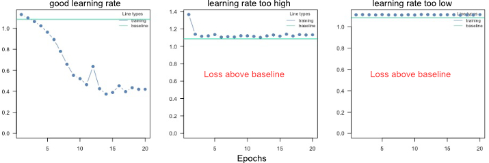
If the training loss of the model doesn't fall below the baseline loss, the learning rate is either too high or too low. If this happens, try higher and lower learning rates.
A common strategy is to try (manually) a few different learning rates to see if the learning rate is on the right scale.
See the troubleshooting vignette (vignette("B-Training_neural_networks")) for more help on training and debugging neural networks.
Finding the right architecture
As with the learning rate, there is no definitive guide to choosing the right architecture for the right task. However, there are some general rules/recommendations: In general, wider, and deeper neural networks can improve generalization - but this is a double-edged sword because it also increases the risk of overfitting. So, if you increase the width and depth of the network, you should also add regularization (e.g., by increasing the lambda parameter, which corresponds to the regularization strength). Furthermore, in Pichler & Hartig, 2023, we investigated the effects of the hyperparameters on the prediction performance as a function of the data size. For example, we found that the selu activation function outperforms relu for small data sizes (<100 observations).
We recommend starting with moderate sizes (like the defaults), and if the model doesn't generalize/converge, try larger networks along with a regularization that helps minimize the risk of overfitting (see vignette("B-Training_neural_networks") ).
Overfitting
Overfitting means that the model fits the training data well, but generalizes poorly to new observations. We can use the validation argument to detect overfitting. If the validation loss starts to increase again at a certain point, it often means that the models are starting to overfit your training data:
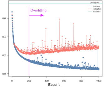
Solutions:
Re-train with epochs = point where model started to overfit
Early stopping, stop training when model starts to overfit, can be specified using the
early_stopping=…argumentUse regularization (dropout or elastic-net, see next section)
Regularization
Elastic Net regularization combines the strengths of L1 (Lasso) and L2 (Ridge) regularization. It introduces a penalty term that encourages sparse weight values while maintaining overall weight shrinkage. By controlling the sparsity of the learned model, Elastic Net regularization helps avoid overfitting while allowing for meaningful feature selection. We advise using elastic net (e.g. lambda = 0.001 and alpha = 0.2).
Dropout regularization helps prevent overfitting by randomly disabling a portion of neurons during training. This technique encourages the network to learn more robust and generalized representations, as it prevents individual neurons from relying too heavily on specific input patterns. Dropout has been widely adopted as a simple yet effective regularization method in deep learning. In the case of 2D and 3D inputs whole feature maps are disabled. Since the torch package doesn't currently support feature map-wise dropout for 1D inputs, instead random neurons in the feature maps are disabled similar to dropout in linear layers.
By utilizing these regularization methods in your neural network training with the cito package, you can improve generalization performance and enhance the network's ability to handle unseen data. These techniques act as valuable tools in mitigating overfitting and promoting more robust and reliable model performance.
Custom Optimizer and Learning Rate Schedulers
When training a network, you have the flexibility to customize the optimizer settings and learning rate scheduler to optimize the learning process. In the cito package, you can initialize these configurations using the config_lr_scheduler and config_optimizer functions.
config_lr_scheduler allows you to define a specific learning rate scheduler that controls how the learning rate changes over time during training. This is beneficial in scenarios where you want to adaptively adjust the learning rate to improve convergence or avoid getting stuck in local optima.
Similarly, the config_optimizer function enables you to specify the optimizer for your network. Different optimizers, such as stochastic gradient descent (SGD), Adam, or RMSprop, offer various strategies for updating the network's weights and biases during training. Choosing the right optimizer can significantly impact the training process and the final performance of your neural network.
Training on graphic cards
If you have an NVIDIA CUDA-enabled device and have installed the CUDA toolkit version 11.3 and cuDNN 8.4, you can take advantage of GPU acceleration for training your neural networks. It is crucial to have these specific versions installed, as other versions may not be compatible. For detailed installation instructions and more information on utilizing GPUs for training, please refer to the mlverse: 'torch' documentation.
Note: GPU training is optional, and the package can still be used for training on CPU even without CUDA and cuDNN installations.
Author(s)
Armin Schenk, Maximilian Pichler
See Also
predict.citocnn, plot.citocnn, coef.citocnn, print.citocnn, summary.citocnn, continue_training, analyze_training
Returns list of parameters the neural network model currently has in use
Description
Returns list of parameters the neural network model currently has in use
Usage
## S3 method for class 'citocnn'
coef(object, ...)
Arguments
object |
a model created by |
... |
nothing implemented yet |
Value
list of weights of neural network
Returns list of parameters the neural network model currently has in use
Description
Returns list of parameters the neural network model currently has in use
Usage
## S3 method for class 'citodnn'
coef(object, ...)

## S3 method for class 'citodnnBootstrap'
coef(object, ...)
Arguments
object |
a model created by |
... |
nothing implemented yet |
Value
list of weights of neural network
Examples
if(torch::torch_is_installed()){
library(cito)

set.seed(222)
validation_set<- sample(c(1:nrow(datasets::iris)),25)

# Build and train  Network
nn.fit<- dnn(Sepal.Length~., data = datasets::iris[-validation_set,])

# Sturcture of Neural Network
print(nn.fit)

#analyze weights of Neural Network
coef(nn.fit)
}
Calculate average conditional effects
Description
Average conditional effects calculate the local derivatives for each observation for each feature. They are similar to marginal effects. And the average of these conditional effects is an approximation of linear effects (see Pichler and Hartig, 2023 for more details). You can use this function to either calculate main effects (on the diagonal, take a look at the example) or interaction effects (off-diagonals) between features.
To obtain uncertainties for these effects, enable the bootstrapping option in the dnn(..) function (see example).
Usage
conditionalEffects(
  object,
  interactions = FALSE,
  epsilon = 0.1,
  device = c("cpu", "cuda", "mps"),
  indices = NULL,
  data = NULL,
  type = "response",
  ...
)

## S3 method for class 'citodnn'
conditionalEffects(
  object,
  interactions = FALSE,
  epsilon = 0.1,
  device = c("cpu", "cuda", "mps"),
  indices = NULL,
  data = NULL,
  type = "response",
  ...
)

## S3 method for class 'citodnnBootstrap'
conditionalEffects(
  object,
  interactions = FALSE,
  epsilon = 0.1,
  device = c("cpu", "cuda", "mps"),
  indices = NULL,
  data = NULL,
  type = "response",
  ...
)
Arguments
object |
object of class |
interactions |
calculate interactions or not (computationally expensive) |
epsilon |
difference used to calculate derivatives |
device |
which device |
indices |
of variables for which the ACE are calculated |
data |
data which is used to calculate the ACE |
type |
ACE on which scale (response or link) |
... |
additional arguments that are passed to the predict function |
Value
an S3 object of class "conditionalEffects" is returned.
The list consists of the following attributes:
result |
3-dimensional array with the raw results |
mean |
Matrix, average conditional effects |
abs |
Matrix, summed absolute conditional effects |
sd |
Matrix, standard deviation of the conditional effects |
Author(s)
Maximilian Pichler
References
Scholbeck, C. A., Casalicchio, G., Molnar, C., Bischl, B., & Heumann, C. (2022). Marginal effects for non-linear prediction functions. arXiv preprint arXiv:2201.08837.
Pichler, M., & Hartig, F. (2023). Can predictive models be used for causal inference?. arXiv preprint arXiv:2306.10551.
Examples
if(torch::torch_is_installed()){
library(cito)

# Build and train  Network
nn.fit = dnn(Sepal.Length~., data = datasets::iris)

# Calculate average conditional effects
ACE = conditionalEffects(nn.fit)

## Main effects (categorical features are not supported)
ACE

## With interaction effects:
ACE = conditionalEffects(nn.fit, interactions = TRUE)
## The off diagonal elements are the interaction effects
ACE[[1]]$mean
## ACE is a list, elements correspond to the number of response classes
## Sepal.length == 1 Response so we have only one
## list element in the ACE object

# Re-train NN with bootstrapping to obtain standard errors
nn.fit = dnn(Sepal.Length~., data = datasets::iris, bootstrap = 30L)
## The summary method calculates also the conditional effects, and if
## bootstrapping was used, it will also report standard errors and p-values:
summary(nn.fit)


}
Creation of customized learning rate scheduler objects
Description
Helps create custom learning rate schedulers for dnn.
Usage
config_lr_scheduler(
  type = c("lambda", "multiplicative", "reduce_on_plateau", "one_cycle", "step"),
  verbose = FALSE,
  ...
)
Arguments
type |
String defining which type of scheduler should be used. See Details. |
verbose |
If TRUE, additional information about scheduler will be printed to console. |
... |
additional arguments to be passed to scheduler. See Details. |
Details
different learning rate scheduler need different variables, these functions will tell you which variables can be set:
lambda:
lr_lambdamultiplicative:
lr_multiplicativereduce_on_plateau:
lr_reduce_on_plateauone_cycle:
lr_one_cyclestep:
lr_step
Value
object of class cito_lr_scheduler to give to dnn
Examples
if(torch::torch_is_installed()){
library(cito)

# create learning rate scheduler object
scheduler <- config_lr_scheduler(type = "step",
                        step_size = 30,
                        gamma = 0.15,
                        verbose = TRUE)

# Build and train  Network
nn.fit<- dnn(Sepal.Length~., data = datasets::iris, lr_scheduler = scheduler)

}
Creation of customized optimizer objects
Description
Helps you create custom optimizer for dnn. It is recommended to set learning rate in dnn.
Usage
config_optimizer(
  type = c("adam", "adadelta", "adagrad", "rmsprop", "rprop", "sgd"),
  verbose = FALSE,
  ...
)
Arguments
type |
character string defining which optimizer should be used. See Details. |
verbose |
If TRUE, additional information about scheduler will be printed to console |
... |
additional arguments to be passed to optimizer. See Details. |
Details
different optimizer need different variables, this function will tell you how the variables are set. For more information see the corresponding functions:
adam:
optim_adamadadelta:
optim_adadeltaadagrad:
optim_adagradrmsprop:
optim_rmsproprprop:
optim_rpropsgd:
optim_sgd
Value
object of class cito_optim to give to dnn
Examples
if(torch::torch_is_installed()){
library(cito)

# create optimizer object
opt <- config_optimizer(type = "adagrad",
                        lr_decay = 1e-04,
                        weight_decay = 0.1,
                        verbose = TRUE)

# Build and train  Network
nn.fit<- dnn(Sepal.Length~., data = datasets::iris, optimizer = opt)

}
Config hyperparameter tuning
Description
Config hyperparameter tuning
Usage
config_tuning(
  CV = 5,
  steps = 10,
  parallel = FALSE,
  NGPU = 1,
  cancel = TRUE,
  bootstrap_final = NULL,
  bootstrap_parallel = FALSE,
  return_models = FALSE
)
Arguments
CV |
numeric, specifies k-folded cross validation |
steps |
numeric, number of random tuning steps |
parallel |
numeric, number of parallel cores (tuning steps are parallelized) |
NGPU |
numeric, set if more than one GPU is available, tuning will be parallelized over CPU cores and GPUs, only works for NCPU > 1 |
cancel |
CV/tuning for specific hyperparameter set if model cannot reduce loss below baseline after burnin or returns NA loss |
bootstrap_final |
bootstrap final model, if all models should be boostrapped it must be set globally via the bootstrap argument in the |
bootstrap_parallel |
should the bootstrapping be parallelized or not |
return_models |
return individual models |
Details
Note that hyperparameter tuning can be expensive. We have implemented an option to parallelize hyperparameter tuning, including parallelization over one or more GPUs (the hyperparameter evaluation is parallelized, not the CV). This can be especially useful for small models. For example, if you have 4 GPUs, 20 CPU cores, and 20 steps (random samples from the random search), you could run ‘dnn(..., device="cuda",lr = tune(), batchsize=tune(), tuning=config_tuning(parallel=20, NGPU=4)’, which will distribute 20 model fits across 4 GPUs, so that each GPU will process 5 models (in parallel).
Continues training of a model generated with dnn or cnn for additional epochs.
Description
If the training/validation loss is still decreasing at the end of the training, it is often a sign that the NN has not yet converged. You can use this function to continue training instead of re-training the entire model.
Usage
continue_training(model, ...)

## S3 method for class 'citodnn'
continue_training(
  model,
  epochs = 32,
  data = NULL,
  device = NULL,
  verbose = TRUE,
  changed_params = NULL,
  ...
)

## S3 method for class 'citodnnBootstrap'
continue_training(
  model,
  epochs = 32,
  data = NULL,
  device = NULL,
  verbose = TRUE,
  changed_params = NULL,
  parallel = FALSE,
  ...
)

## S3 method for class 'citocnn'
continue_training(
  model,
  epochs = 32,
  X = NULL,
  Y = NULL,
  device = c("cpu", "cuda", "mps"),
  verbose = TRUE,
  changed_params = NULL,
  ...
)
Arguments
model |
|
... |
class-specific arguments |
epochs |
additional epochs the training should continue for |
data |
matrix or data.frame. If not provided data from original training will be used |
device |
can be used to overwrite device used in previous training |
verbose |
print training and validation loss of epochs |
changed_params |
list of arguments to change compared to original training setup, see |
parallel |
train bootstrapped model in parallel |
X |
array. If not provided X from original training will be used |
Y |
vector, factor, numerical matrix or logical matrix. If not provided Y from original training will be used |
Value
a model of class citodnn, citodnnBootstrap or citocnn created by dnn or cnn
Examples
if(torch::torch_is_installed()){
library(cito)

set.seed(222)
validation_set<- sample(c(1:nrow(datasets::iris)),25)

# Build and train  Network
nn.fit<- dnn(Sepal.Length~., data = datasets::iris[-validation_set,], epochs = 32)

# continue training for another 32 epochs
nn.fit<- continue_training(nn.fit,epochs = 32)

# Use model on validation set
predictions <- predict(nn.fit, iris[validation_set,])
}
Convolutional layer
Description
creates a 'conv' 'citolayer' object that is used by create_architecture.
Usage
conv(
  n_kernels = NULL,
  kernel_size = NULL,
  stride = NULL,
  padding = NULL,
  dilation = NULL,
  bias = NULL,
  activation = NULL,
  normalization = NULL,
  dropout = NULL
)
Arguments
n_kernels |
(int) amount of kernels in this layer |
kernel_size |
(int or tuple) size of the kernels in this layer. Use a tuple if the kernel size isn't equal in all dimensions |
stride |
(int or tuple) stride of the kernels in this layer. NULL sets the stride equal to the kernel size. Use a tuple if the stride isn't equal in all dimensions |
padding |
(int or tuple) zero-padding added to both sides of the input. Use a tuple if the padding isn't equal in all dimensions |
dilation |
(int or tuple) dilation of the kernels in this layer. Use a tuple if the dilation isn't equal in all dimensions |
bias |
(boolean) if TRUE, adds a learnable bias to the kernels of this layer |
activation |
(string) activation function that is used after this layer. The following activation functions are supported: "relu", "leaky_relu", "tanh", "elu", "rrelu", "prelu", "softplus", "celu", "selu", "gelu", "relu6", "sigmoid", "softsign", "hardtanh", "tanhshrink", "softshrink", "hardshrink", "log_sigmoid" |
normalization |
(boolean) if TRUE, batch normalization is used after this layer |
dropout |
(float) dropout rate of this layer. Set to 0 for no dropout |
Details
This function creates a 'conv' 'citolayer' object that is passed to the create_architecture function.
The parameters that aren't assigned here (and are therefore still NULL) are filled with the default values passed to create_architecture.
Value
S3 object of class "conv" "citolayer"
Author(s)
Armin Schenk
See Also
CNN architecture
Description
creates a 'citoarchitecture' object that is used by cnn.
Usage
create_architecture(
  ...,
  default_n_neurons = 10,
  default_n_kernels = 10,
  default_kernel_size = list(conv = 3, maxPool = 2, avgPool = 2),
  default_stride = list(conv = 1, maxPool = NULL, avgPool = NULL),
  default_padding = list(conv = 0, maxPool = 0, avgPool = 0),
  default_dilation = list(conv = 1, maxPool = 1),
  default_bias = list(conv = TRUE, linear = TRUE),
  default_activation = list(conv = "relu", linear = "relu"),
  default_normalization = list(conv = FALSE, linear = FALSE),
  default_dropout = list(conv = 0, linear = 0)
)
Arguments
... |
objects of class 'citolayer' created by |
default_n_neurons |
(int) default value: amount of neurons in a linear layer |
default_n_kernels |
(int) default value: amount of kernels in a convolutional layer |
default_kernel_size |
(int or tuple) default value: size of the kernels in convolutional and pooling layers. Use a tuple if the kernel size isn't equal in all dimensions |
default_stride |
(int or tuple) default value: stride of the kernels in convolutional and pooling layers. NULL sets the stride equal to the kernel size. Use a tuple if the stride isn't equal in all dimensions |
default_padding |
(int or tuple) default value: zero-padding added to both sides of the input. Use a tuple if the padding isn't equal in all dimensions |
default_dilation |
(int or tuple) default value: dilation of the kernels in convolutional and maxPooling layers. Use a tuple if the dilation isn't equal in all dimensions |
default_bias |
(boolean) default value: if TRUE, adds a learnable bias to neurons of linear and kernels of convolutional layers |
default_activation |
(string) default value: activation function that is used after linear and convolutional layers. The following activation functions are supported: "relu", "leaky_relu", "tanh", "elu", "rrelu", "prelu", "softplus", "celu", "selu", "gelu", "relu6", "sigmoid", "softsign", "hardtanh", "tanhshrink", "softshrink", "hardshrink", "log_sigmoid" |
default_normalization |
(boolean) default value: if TRUE, batch normalization is used after linear and convolutional layers |
default_dropout |
(float) default value: dropout rate of linear and convolutional layers. Set to 0 for no dropout |
Details
This function creates a 'citoarchitecture' object that provides the cnn function with all information about the architecture of the CNN that will be created and trained.
The final architecture consists of the layers in the sequence they were passed to this function.
All parameters of the 'citolayer' objects, that are still NULL because they haven't been specified at the creation of the layer, are filled with the given default parameters for their specific layer type (linear, conv, maxPool, avgPool).
The default values can be changed by either passing a list with the values for specific layer types (in which case the defaults of layer types which aren't in the list remain the same)
or by passing a single value (in which case the defaults for all layer types is set to that value).
Value
S3 object of class "citoarchitecture"
Author(s)
Armin Schenk
See Also
cnn, linear, conv, maxPool, avgPool, transfer, print.citoarchitecture, plot.citoarchitecture
DNN
Description
fits a custom deep neural network using the Multilayer Perceptron architecture. dnn() supports the formula syntax and allows to customize the neural network to a maximal degree.
Usage
dnn(
  formula = NULL,
  data = NULL,
  hidden = c(50L, 50L),
  activation = "selu",
  bias = TRUE,
  dropout = 0,
  loss = c("mse", "mae", "softmax", "cross-entropy", "gaussian", "binomial", "poisson",
    "mvp", "nbinom"),
  validation = 0,
  lambda = 0,
  alpha = 0.5,
  optimizer = c("sgd", "adam", "adadelta", "adagrad", "rmsprop", "rprop"),
  lr = 0.01,
  batchsize = NULL,
  burnin = 30,
  baseloss = NULL,
  shuffle = TRUE,
  epochs = 100,
  bootstrap = NULL,
  bootstrap_parallel = FALSE,
  plot = TRUE,
  verbose = TRUE,
  lr_scheduler = NULL,
  custom_parameters = NULL,
  device = c("cpu", "cuda", "mps"),
  early_stopping = FALSE,
  tuning = config_tuning(),
  X = NULL,
  Y = NULL
)
Arguments
formula |
an object of class " |
data |
matrix or data.frame with features/predictors and response variable |
|
hidden units in layers, length of hidden corresponds to number of layers | |
activation |
activation functions, can be of length one, or a vector of different activation functions for each layer |
bias |
whether use biases in the layers, can be of length one, or a vector (number of hidden layers + 1 (last layer)) of logicals for each layer. |
dropout |
dropout rate, probability of a node getting left out during training (see |
loss |
loss after which network should be optimized. Can also be distribution from the stats package or own function, see details |
validation |
percentage of data set that should be taken as validation set (chosen randomly) |
lambda |
strength of regularization: lambda penalty, |
alpha |
add L1/L2 regularization to training |
optimizer |
which optimizer used for training the network, for more adjustments to optimizer see |
lr |
learning rate given to optimizer |
batchsize |
number of samples that are used to calculate one learning rate step, default is 10% of the training data |
burnin |
training is aborted if the trainings loss is not below the baseline loss after burnin epochs |
baseloss |
baseloss, if null baseloss corresponds to intercept only models |
shuffle |
if TRUE, data in each batch gets reshuffled every epoch |
epochs |
epochs the training goes on for |
bootstrap |
bootstrap neural network or not, numeric corresponds to number of bootstrap samples |
bootstrap_parallel |
parallelize (CPU) bootstrapping |
plot |
plot training loss |
verbose |
print training and validation loss of epochs |
lr_scheduler |
learning rate scheduler created with |
custom_parameters |
List of parameters/variables to be optimized. Can be used in a custom loss function. See Vignette for example. |
device |
device on which network should be trained on. mps correspond to M1/M2 GPU devices. |
early_stopping |
if set to integer, training will stop if loss has gotten higher for defined number of epochs in a row, will use validation loss is available. |
tuning |
tuning options created with |
X |
Feature matrix or data.frame, alternative data interface |
Y |
Response vector, factor, matrix or data.frame, alternative data interface |
Value
an S3 object of class "cito.dnn" is returned. It is a list containing everything there is to know about the model and its training process.
The list consists of the following attributes:
net |
An object of class "nn_sequential" "nn_module", originates from the torch package and represents the core object of this workflow. |
call |
The original function call |
loss |
A list which contains relevant information for the target variable and the used loss function |
data |
Contains data used for training the model |
weigths |
List of weights for each training epoch |
use_model_epoch |
Integer, which defines which model from which training epoch should be used for prediction. 1 = best model, 2 = last model |
loaded_model_epoch |
Integer, shows which model from which epoch is loaded currently into model$net. |
model_properties |
A list of properties of the neural network, contains number of input nodes, number of output nodes, size of hidden layers, activation functions, whether bias is included and if dropout layers are included. |
training_properties |
A list of all training parameters that were used the last time the model was trained. It consists of learning rate, information about an learning rate scheduler, information about the optimizer, number of epochs, whether early stopping was used, if plot was active, lambda and alpha for L1/L2 regularization, batchsize, shuffle, was the data set split into validation and training, which formula was used for training and at which epoch did the training stop. |
losses |
A data.frame containing training and validation losses of each epoch |
Activation functions
Supported activation functions: "relu", "leaky_relu", "tanh", "elu", "rrelu", "prelu", "softplus", "celu", "selu", "gelu", "relu6", "sigmoid", "softsign", "hardtanh", "tanhshrink", "softshrink", "hardshrink", "log_sigmoid"
Loss functions / Likelihoods
We support loss functions and likelihoods for different tasks:
| Name | Explanation | Example / Task |
| mse | mean squared error | Regression, predicting continuous values |
| mae | mean absolute error | Regression, predicting continuous values |
| softmax | categorical cross entropy | Multi-class, species classification |
| cross-entropy | categorical cross entropy | Multi-class, species classification |
| gaussian | Normal likelihood | Regression, residual error is also estimated (similar to stats::lm()) |
| binomial | Binomial likelihood | Classification/Logistic regression, mortality |
| poisson | Poisson likelihood | Regression, count data, e.g. species abundances |
| nbinom | Negative binomial likelihood | Regression, count data with dispersion parameter |
| mvp | multivariate probit model | joint species distribution model, multi species (presence absence) |
Training and convergence of neural networks
Ensuring convergence can be tricky when training neural networks. Their training is sensitive to a combination of the learning rate (how much the weights are updated in each optimization step), the batch size (a random subset of the data is used in each optimization step), and the number of epochs (number of optimization steps). Typically, the learning rate should be decreased with the size of the neural networks (depth of the network and width of the hidden layers). We provide a baseline loss (intercept only model) that can give hints about an appropriate learning rate:
If the training loss of the model doesn't fall below the baseline loss, the learning rate is either too high or too low. If this happens, try higher and lower learning rates.
A common strategy is to try (manually) a few different learning rates to see if the learning rate is on the right scale.
See the troubleshooting vignette (vignette("B-Training_neural_networks")) for more help on training and debugging neural networks.
Finding the right architecture
As with the learning rate, there is no definitive guide to choosing the right architecture for the right task. However, there are some general rules/recommendations: In general, wider, and deeper neural networks can improve generalization - but this is a double-edged sword because it also increases the risk of overfitting. So, if you increase the width and depth of the network, you should also add regularization (e.g., by increasing the lambda parameter, which corresponds to the regularization strength). Furthermore, in Pichler & Hartig, 2023, we investigated the effects of the hyperparameters on the prediction performance as a function of the data size. For example, we found that the selu activation function outperforms relu for small data sizes (<100 observations).
We recommend starting with moderate sizes (like the defaults), and if the model doesn't generalize/converge, try larger networks along with a regularization that helps minimize the risk of overfitting (see vignette("B-Training_neural_networks") ).
Overfitting
Overfitting means that the model fits the training data well, but generalizes poorly to new observations. We can use the validation argument to detect overfitting. If the validation loss starts to increase again at a certain point, it often means that the models are starting to overfit your training data:
Solutions:
Re-train with epochs = point where model started to overfit
Early stopping, stop training when model starts to overfit, can be specified using the
early_stopping=…argumentUse regularization (dropout or elastic-net, see next section)
Regularization
Elastic Net regularization combines the strengths of L1 (Lasso) and L2 (Ridge) regularization. It introduces a penalty term that encourages sparse weight values while maintaining overall weight shrinkage. By controlling the sparsity of the learned model, Elastic Net regularization helps avoid overfitting while allowing for meaningful feature selection. We advise using elastic net (e.g. lambda = 0.001 and alpha = 0.2).
Dropout regularization helps prevent overfitting by randomly disabling a portion of neurons during training. This technique encourages the network to learn more robust and generalized representations, as it prevents individual neurons from relying too heavily on specific input patterns. Dropout has been widely adopted as a simple yet effective regularization method in deep learning.
By utilizing these regularization methods in your neural network training with the cito package, you can improve generalization performance and enhance the network's ability to handle unseen data. These techniques act as valuable tools in mitigating overfitting and promoting more robust and reliable model performance.
Uncertainty
We can use bootstrapping to generate uncertainties for all outputs. Bootstrapping can be enabled by setting bootstrap = ... to the number of bootstrap samples to be used. Note, however, that the computational cost can be excessive.
In some cases it may be worthwhile to parallelize bootstrapping, for example if you have a GPU and the neural network is small. Parallelization for bootstrapping can be enabled by setting the bootstrap_parallel = ... argument to the desired number of calls to run in parallel.
Custom Optimizer and Learning Rate Schedulers
When training a network, you have the flexibility to customize the optimizer settings and learning rate scheduler to optimize the learning process. In the cito package, you can initialize these configurations using the config_lr_scheduler and config_optimizer functions.
config_lr_scheduler allows you to define a specific learning rate scheduler that controls how the learning rate changes over time during training. This is beneficial in scenarios where you want to adaptively adjust the learning rate to improve convergence or avoid getting stuck in local optima.
Similarly, the config_optimizer function enables you to specify the optimizer for your network. Different optimizers, such as stochastic gradient descent (SGD), Adam, or RMSprop, offer various strategies for updating the network's weights and biases during training. Choosing the right optimizer can significantly impact the training process and the final performance of your neural network.
Hyperparameter tuning
We have implemented experimental support for hyperparameter tuning. We can mark hyperparameters that should be tuned by cito by setting their values to tune(), for example dnn (..., lr = tune(). tune() is a function that creates a range of random values for the given hyperparameter. You can change the maximum and minimum range of the potential hyperparameters or pass custom values to the tune(values = c(....)) function. The following table lists the hyperparameters that can currently be tuned:
| Hyperparameter | Example | Details |
| hidden | dnn(…,hidden=tune(10, 20, fixed=’depth’)) | Depth and width can be both tuned or only one of them, if both of them should be tuned, vectors for lower and upper #' boundaries must be provided (first = number of nodes) |
| bias | dnn(…, bias=tune()) | Should the bias be turned on or off for all hidden layers |
| lambda | dnn(…, lambda = tune(0.0001, 0.1)) | lambda will be tuned within the range (0.0001, 0.1) |
| alpha | dnn(…, lambda = tune(0.2, 0.4)) | alpha will be tuned within the range (0.2, 0.4) |
| activation | dnn(…, activation = tune()) | activation functions of the hidden layers will be tuned |
| dropout | dnn(…, dropout = tune()) | Dropout rate will be tuned (globally for all layers) |
| lr | dnn(…, lr = tune()) | Learning rate will be tuned |
| batchsize | dnn(…, batchsize = tune()) | batch size will be tuned |
| epochs | dnn(…, batchsize = tune()) | batchsize will be tuned |
The hyperparameters are tuned by random search (i.e., random values for the hyperparameters within a specified range) and by cross-validation. The exact tuning regime can be specified with config_tuning.
Note that hyperparameter tuning can be expensive. We have implemented an option to parallelize hyperparameter tuning, including parallelization over one or more GPUs (the hyperparameter evaluation is parallelized, not the CV). This can be especially useful for small models. For example, if you have 4 GPUs, 20 CPU cores, and 20 steps (random samples from the random search), you could run dnn(..., device="cuda",lr = tune(), batchsize=tune(), tuning=config_tuning(parallel=20, NGPU=4), which will distribute 20 model fits across 4 GPUs, so that each GPU will process 5 models (in parallel).
As this is an experimental feature, we welcome feature requests and bug reports on our github site.
For the custom values, all hyperparameters except for the hidden layers require a vector of values. Hidden layers expect a two-column matrix where the first column is the number of hidden nodes and the second column corresponds to the number of hidden layers.
How neural networks work
In Multilayer Perceptron (MLP) networks, each neuron is connected to every neuron in the previous layer and every neuron in the subsequent layer. The value of each neuron is computed using a weighted sum of the outputs from the previous layer, followed by the application of an activation function. Specifically, the value of a neuron is calculated as the weighted sum of the outputs of the neurons in the previous layer, combined with a bias term. This sum is then passed through an activation function, which introduces non-linearity into the network. The calculated value of each neuron becomes the input for the neurons in the next layer, and the process continues until the output layer is reached. The choice of activation function and the specific weight values determine the network's ability to learn and approximate complex relationships between inputs and outputs.
Therefore the value of each neuron can be calculated using: a (\sum_j{ w_j * a_j}). Where w_j is the weight and a_j is the value from neuron j to the current one. a() is the activation function, e.g. relu(x) = max(0,x)
Training on graphic cards
If you have an NVIDIA CUDA-enabled device and have installed the CUDA toolkit version 11.3 and cuDNN 8.4, you can take advantage of GPU acceleration for training your neural networks. It is crucial to have these specific versions installed, as other versions may not be compatible. For detailed installation instructions and more information on utilizing GPUs for training, please refer to the mlverse: 'torch' documentation.
Note: GPU training is optional, and the package can still be used for training on CPU even without CUDA and cuDNN installations.
Author(s)
Christian Amesoeder, Maximilian Pichler
See Also
predict.citodnn, plot.citodnn, coef.citodnn,print.citodnn, summary.citodnn, continue_training, analyze_training, PDP, ALE,
Examples
if(torch::torch_is_installed()){
library(cito)

# Example workflow in cito

## Build and train  Network
### softmax is used for multi-class responses (e.g., Species)
nn.fit<- dnn(Species~., data = datasets::iris, loss = "softmax")

## The training loss is below the baseline loss but at the end of the
## training the loss was still decreasing, so continue training for another 50
## epochs
nn.fit <- continue_training(nn.fit, epochs = 50L)

# Sturcture of Neural Network
print(nn.fit)

# Plot Neural Network
plot(nn.fit)
## 4 Input nodes (first layer) because of 4 features
## 3 Output nodes (last layer) because of 3 response species (one node for each
## level in the response variable).
## The layers between the input and output layer are called hidden layers (two
## of them)

## We now want to understand how the predictions are made, what are the
## important features? The summary function automatically calculates feature
## importance (the interpretation is similar to an anova) and calculates
## average conditional effects that are similar to linear effects:
summary(nn.fit)

## To visualize the effect (response-feature effect), we can use the ALE and
## PDP functions

# Partial dependencies
PDP(nn.fit, variable = "Petal.Length")

# Accumulated local effect plots
ALE(nn.fit, variable = "Petal.Length")


# Per se, it is difficult to get confidence intervals for our xAI metrics (or
# for the predictions). But we can use bootstrapping to obtain uncertainties
# for all cito outputs:
## Re-fit the neural network with bootstrapping
nn.fit<- dnn(Species~.,
             data = datasets::iris,
             loss = "softmax",
             epochs = 150L,
             verbose = FALSE,
             bootstrap = 20L)
## convergence can be tested via the analyze_training function
analyze_training(nn.fit)

## Summary for xAI metrics (can take some time):
summary(nn.fit)
## Now with standard errors and p-values
## Note: Take the p-values with a grain of salt! We do not know yet if they are
## correct (e.g. if you use regularization, they are likely conservative == too
## large)

## Predictions with bootstrapping:
dim(predict(nn.fit))
## predictions are by default averaged (over the bootstrap samples)


# Hyperparameter tuning (experimental feature)
hidden_values = matrix(c(5, 2,
                         4, 2,
                         10,2,
                         15,2), 4, 2, byrow = TRUE)
## Potential architectures we want to test, first column == number of nodes
print(hidden_values)

nn.fit = dnn(Species~.,
             data = iris,
             epochs = 30L,
             loss = "softmax",
             hidden = tune(values = hidden_values),
             lr = tune(0.00001, 0.1) # tune lr between range 0.00001 and 0.1
             )
## Tuning results:
print(nn.fit$tuning)

# test = Inf means that tuning was cancelled after only one fit (within the CV)


# Advanced: Custom loss functions and additional parameters
## Normal Likelihood with sd parameter:
custom_loss = function(pred, true) {
  logLik = torch::distr_normal(pred,
                               scale = torch::nnf_relu(scale)+
                                 0.001)$log_prob(true)
  return(-logLik$mean())
}

nn.fit<- dnn(Sepal.Length~.,
             data = datasets::iris,
             loss = custom_loss,
             verbose = FALSE,
             custom_parameters = list(scale = 1.0)
)
nn.fit$parameter$scale

## Multivariate normal likelihood with parametrized covariance matrix
## Sigma = L*L^t + D
## Helper function to build covariance matrix
create_cov = function(LU, Diag) {
  return(torch::torch_matmul(LU, LU$t()) + torch::torch_diag(Diag$exp()+0.01))
}

custom_loss_MVN = function(true, pred) {
  Sigma = create_cov(SigmaPar, SigmaDiag)
  logLik = torch::distr_multivariate_normal(pred,
                                            covariance_matrix = Sigma)$
    log_prob(true)
  return(-logLik$mean())
}


nn.fit<- dnn(cbind(Sepal.Length, Sepal.Width, Petal.Length)~.,
             data = datasets::iris,
             lr = 0.01,
             verbose = FALSE,
             loss = custom_loss_MVN,
             custom_parameters =
               list(SigmaDiag =  rep(0, 3),
                    SigmaPar = matrix(rnorm(6, sd = 0.001), 3, 2))
)
as.matrix(create_cov(nn.fit$loss$parameter$SigmaPar,
                     nn.fit$loss$parameter$SigmaDiag))

}
Embeddings
Description
Can be used for categorical variables, a more efficient alternative to one-hot encoding
Usage
e(dim = 1L, weights = NULL, train = TRUE, lambda = 0, alpha = 1)
Arguments
dim |
integer, embedding dimension |
weights |
matrix, to use custom embedding matrices |
train |
logical, should the embeddings be trained or not |
lambda |
regularization strength on the embeddings |
alpha |
mix between L1 and L2 regularization |
list of specials – taken from enum.R
Description
list of specials – taken from enum.R
Usage
findReTrmClasses()
Linear layer
Description
creates a 'linear' 'citolayer' object that is used by create_architecture.
Usage
linear(
  n_neurons = NULL,
  bias = NULL,
  activation = NULL,
  normalization = NULL,
  dropout = NULL
)
Arguments
n_neurons |
(int) amount of hidden neurons in this layer |
bias |
(boolean) if TRUE, adds a learnable bias to the neurons of this layer |
activation |
(string) activation function that is used after this layer. The following activation functions are supported: "relu", "leaky_relu", "tanh", "elu", "rrelu", "prelu", "softplus", "celu", "selu", "gelu", "relu6", "sigmoid", "softsign", "hardtanh", "tanhshrink", "softshrink", "hardshrink", "log_sigmoid" |
normalization |
(boolean) if TRUE, batch normalization is used after this layer |
dropout |
(float) dropout rate of this layer. Set to 0 for no dropout |
Details
This function creates a 'linear' 'citolayer' object that is passed to the create_architecture function.
The parameters that aren't assigned here (and are therefore still NULL) are filled with the default values passed to create_architecture.
Value
S3 object of class "linear" "citolayer"
Author(s)
Armin Schenk
See Also
Maximum pooling layer
Description
creates a 'maxPool' 'citolayer' object that is used by create_architecture.
Usage
maxPool(kernel_size = NULL, stride = NULL, padding = NULL, dilation = NULL)
Arguments
kernel_size |
(int or tuple) size of the kernel in this layer. Use a tuple if the kernel size isn't equal in all dimensions |
stride |
(int or tuple) stride of the kernel in this layer. NULL sets the stride equal to the kernel size. Use a tuple if the stride isn't equal in all dimensions |
padding |
(int or tuple) zero-padding added to both sides of the input. Use a tuple if the padding isn't equal in all dimensions |
dilation |
(int or tuple) dilation of the kernel in this layer. Use a tuple if the dilation isn't equal in all dimensions |
Details
This function creates a 'maxPool' 'citolayer' object that is passed to the create_architecture function.
The parameters that aren't assigned here (and are therefore still NULL) are filled with the default values passed to create_architecture.
Value
S3 object of class "maxPool" "citolayer"
Author(s)
Armin Schenk
See Also
Plot the CNN architecture
Description
Plot the CNN architecture
Usage
## S3 method for class 'citoarchitecture'
plot(x, input_shape, output_shape, ...)
Arguments
x |
an object of class citoarchitecture created by |
input_shape |
a vector with the dimensions of a single sample (e.g. c(3,28,28)) |
output_shape |
the number of nodes in the output layer |
... |
additional arguments |
Value
nothing
Plot the CNN architecture
Description
Plot the CNN architecture
Usage
## S3 method for class 'citocnn'
plot(x, ...)
Arguments
x |
a model created by |
... |
additional arguments |
Value
original object x
Creates graph plot which gives an overview of the network architecture.
Description
Creates graph plot which gives an overview of the network architecture.
Usage
## S3 method for class 'citodnn'
plot(x, node_size = 1, scale_edges = FALSE, ...)

## S3 method for class 'citodnnBootstrap'
plot(x, node_size = 1, scale_edges = FALSE, which_model = 1, ...)
Arguments
x |
a model created by |
node_size |
size of node in plot |
scale_edges |
edge weight gets scaled according to other weights (layer specific) |
... |
no further functionality implemented yet |
which_model |
which model from the ensemble should be plotted |
Value
A plot made with 'ggraph' + 'igraph' that represents the neural network
Examples
if(torch::torch_is_installed()){
library(cito)

set.seed(222)
validation_set<- sample(c(1:nrow(datasets::iris)),25)

# Build and train  Network
nn.fit<- dnn(Sepal.Length~., data = datasets::iris[-validation_set,])

plot(nn.fit)
}
Predict from a fitted cnn model
Description
Predict from a fitted cnn model
Usage
## S3 method for class 'citocnn'
predict(
  object,
  newdata = NULL,
  type = c("link", "response", "class"),
  device = c("cpu", "cuda", "mps"),
  ...
)
Arguments
object |
a model created by |
newdata |
new data for predictions |
type |
which value should be calculated, either raw response, output of link function or predicted class (in case of classification) |
device |
device on which network should be trained on. |
... |
additional arguments |
Value
prediction matrix
Predict from a fitted dnn model
Description
Predict from a fitted dnn model
Usage
## S3 method for class 'citodnn'
predict(
  object,
  newdata = NULL,
  type = c("link", "response", "class"),
  device = c("cpu", "cuda", "mps"),
  reduce = c("mean", "median", "none"),
  ...
)

## S3 method for class 'citodnnBootstrap'
predict(
  object,
  newdata = NULL,
  type = c("link", "response", "class"),
  device = c("cpu", "cuda", "mps"),
  reduce = c("mean", "median", "none"),
  ...
)
Arguments
object |
a model created by |
newdata |
new data for predictions |
type |
type of predictions. The default is on the scale of the linear predictor, "response" is on the scale of the response, and "class" means that class predictions are returned (if it is a classification task) |
device |
device on which network should be trained on. |
reduce |
predictions from bootstrapped model are by default reduced (mean, optional median or none) |
... |
additional arguments |
Value
prediction matrix
Examples
if(torch::torch_is_installed()){
library(cito)

set.seed(222)
validation_set<- sample(c(1:nrow(datasets::iris)),25)

# Build and train  Network
nn.fit<- dnn(Sepal.Length~., data = datasets::iris[-validation_set,])

# Use model on validation set
predictions <- predict(nn.fit, iris[validation_set,])
# Scatterplot
plot(iris[validation_set,]$Sepal.Length,predictions)
# MAE
mean(abs(predictions-iris[validation_set,]$Sepal.Length))
}
Print pooling layer
Description
Print pooling layer
Usage
## S3 method for class 'avgPool'
print(x, input_shape, ...)
Arguments
x |
an object of class avgPool |
input_shape |
input shape |
... |
further arguments, not supported yet |
Print class citoarchitecture
Description
Print class citoarchitecture
Usage
## S3 method for class 'citoarchitecture'
print(x, input_shape, output_shape, ...)
Arguments
x |
an object created by |
input_shape |
a vector with the dimensions of a single sample (e.g. c(3,28,28)) |
output_shape |
the number of nodes in the output layer |
... |
additional arguments |
Value
original object
Print class citocnn
Description
Print class citocnn
Usage
## S3 method for class 'citocnn'
print(x, ...)
Arguments
x |
a model created by |
... |
additional arguments |
Value
original object x
Print class citodnn
Description
Print class citodnn
Usage
## S3 method for class 'citodnn'
print(x, ...)

## S3 method for class 'citodnnBootstrap'
print(x, ...)
Arguments
x |
a model created by |
... |
additional arguments |
Value
original object x gets returned
Examples
if(torch::torch_is_installed()){
library(cito)

set.seed(222)
validation_set<- sample(c(1:nrow(datasets::iris)),25)

# Build and train  Network
nn.fit<- dnn(Sepal.Length~., data = datasets::iris[-validation_set,])

# Structure of Neural Network
print(nn.fit)
}
Print average conditional effects
Description
Print average conditional effects
Usage
## S3 method for class 'conditionalEffects'
print(x, ...)

## S3 method for class 'conditionalEffectsBootstrap'
print(x, ...)
Arguments
x |
print ACE calculated by |
... |
optional arguments for compatibility with the generic function, no function implemented |
Value
Matrix with average conditional effects
Print conv layer
Description
Print conv layer
Usage
## S3 method for class 'conv'
print(x, input_shape, ...)
Arguments
x |
an object of class conv |
input_shape |
input shape |
... |
further arguments, not supported yet |
Print linear layer
Description
Print linear layer
Usage
## S3 method for class 'linear'
print(x, input_shape, ...)
Arguments
x |
an object of class linear |
input_shape |
input shape |
... |
further arguments, not supported yet |
Print pooling layer
Description
Print pooling layer
Usage
## S3 method for class 'maxPool'
print(x, input_shape, ...)
Arguments
x |
an object of class maxPool |
input_shape |
input shape |
... |
further arguments, not supported yet |
Print method for class summary.citodnn
Description
Print method for class summary.citodnn
Usage
## S3 method for class 'summary.citodnn'
print(x, ...)

## S3 method for class 'summary.citodnnBootstrap'
print(x, ...)
Arguments
x |
a summary object created by |
... |
additional arguments |
Value
List with Matrices for importance, average CE, absolute sum of CE, and standard deviation of the CE
Print transfer model
Description
Print transfer model
Usage
## S3 method for class 'transfer'
print(x, input_shape, output_shape, ...)
Arguments
x |
an object of class transfer |
input_shape |
input shape |
output_shape |
output shape |
... |
further arguments, not supported yet |
Extract Model Residuals
Description
Returns residuals of training set.
Usage
## S3 method for class 'citodnn'
residuals(object, ...)
Arguments
object |
a model created by |
... |
no additional arguments implemented |
Value
residuals of training set
Data Simulation for CNN
Description
generates images of rectangles and ellipsoids
Usage
simulate_shapes(n, size, channels = 1)
Arguments
n |
number of images |
size |
size of the (quadratic) images |
channels |
number of channels the generated data has (in each channel a new rectangle/ellipsoid is created) |
Details
This function generates simple data to demonstrate the usage of cnn(). The generated images are of centered rectangles and ellipsoids with random widths and heights.
Value
array of dimension (n, 1, size, size)
Author(s)
Armin Schenk
combine a list of formula terms as a sum
Description
combine a list of formula terms as a sum
Usage
sumTerms(termList)
Arguments
termList |
a list of formula terms |
Summary citocnn
Description
currently the same as the print.citocnn method.
Usage
## S3 method for class 'citocnn'
summary(object, ...)
Arguments
object |
a model created by |
... |
additional arguments |
Value
original object x
Summarize Neural Network of class citodnn
Description
Performs a Feature Importance calculation based on Permutations
Usage
## S3 method for class 'citodnn'
summary(object, n_permute = NULL, device = NULL, ...)

## S3 method for class 'citodnnBootstrap'
summary(object, n_permute = NULL, device = NULL, adjust_se = FALSE, ...)
Arguments
object |
a model of class citodnn created by |
n_permute |
number of permutations performed. Default is |
device |
for calculating variable importance and conditional effects |
... |
additional arguments |
adjust_se |
adjust standard errors for importance (standard errors are multiplied with 1/sqrt(3) ) |
Details
Performs the feature importance calculation as suggested by Fisher, Rudin, and Dominici (2018), and the mean and standard deviation of the average conditional Effects as suggested by Pichler & Hartig (2023).
Feature importances are in their interpretation similar to a ANOVA. Main and interaction effects are absorbed into the features. Also, feature importances are prone to collinearity between features, i.e. if two features are collinear, the importances might be overestimated.
Average conditional effects (ACE) are similar to marginal effects and approximate linear effects, i.e. their interpretation is similar to effects in a linear regression model.
The standard deviation of the ACE informs about the non-linearity of the feature effects. Higher values correlate with stronger non-linearities.
For each feature n permutation get done and original and permuted predictive mean squared error (e_{perm} & e_{orig}) get evaluated with FI_j= e_{perm}/e_{orig}. Based on Mean Squared Error.
Value
summary.citodnn returns an object of class "summary.citodnn", a list with components
Transfer learning
Description
creates a 'transfer' 'citolayer' object that is used by create_architecture.
Usage
transfer(
  name = c("alexnet", "inception_v3", "mobilenet_v2", "resnet101", "resnet152",
    "resnet18", "resnet34", "resnet50", "resnext101_32x8d", "resnext50_32x4d", "vgg11",
    "vgg11_bn", "vgg13", "vgg13_bn", "vgg16", "vgg16_bn", "vgg19", "vgg19_bn",
    "wide_resnet101_2", "wide_resnet50_2"),
  pretrained = TRUE,
  freeze = TRUE
)
Arguments
name |
The name of the pretrained model |
pretrained |
if FALSE, random weights are used instead of the pretrained weights |
freeze |
if TRUE, the weights of the pretrained model (except the "classifier" part at the end) aren't changed in the training anymore. Only works if pretrained=TRUE |
Details
This function creates a 'transfer' 'citolayer' object that is passed to the create_architecture function.
With this object the pretrained models that are available in the 'torchvision' package can be used in cito.
When 'freeze' is set to TRUE, only the weights of the last part of the network (consisting of one or more linear layers) are adjusted in the training.
There mustn't be any other citolayers before the transfer citolayer object when calling create_architecture.
If there are any citolayers after the transfer citolayer, the linear classifier part of the pretrained model is replaced with the specified citolayers.
Value
S3 object of class "transfer" "citolayer"
Author(s)
Armin Schenk
See Also
Tune hyperparameter
Description
Control hyperparameter tuning
Usage
tune(
  lower = NULL,
  upper = NULL,
  fixed = NULL,
  additional = NULL,
  values = NULL
)
Arguments
lower |
numeric, numeric vector, character, lower boundaries of tuning space |
upper |
numeric, numeric vector, character, upper boundaries of tuning space |
fixed |
character, used for multi-dimensional hyperparameters such as hidden, which dimensions should be fixed |
additional |
numeric, additional control parameter which sets the value of the fixed argument |
values |
custom values from which hyperparameters are sampled, must be a matrix for hidden layers (first column == nodes, second column == number of layers) |